Post-event aerial imagery tiles

Saved results from a run against the live service; the notebook records when it ran and the checksums of what it read. Run it yourself.

After a hurricane, flood, fire, or tornado, NOAA's National Geodetic Survey flies the damaged area, mosaics its aerial photographs, and cuts the mosaic into GeoTIFF tiles, which it publishes in the public noaa-eri-pds S3 bucket. One file is one tile of one flight: red, green, and blue at 15 to 35 cm per pixel, over a square about 1.4 to 2.8 km on a side, named for its north-west corner. Of the bucket's 52 events, only three are tornadoes.

This walkthrough takes the tile over Germantown, just north of downtown Nashville, from the flight NGS made four days after the tornado of 3 March 2020. usdata has no GeoTIFF reader, so the notebook opens the file's built-in overviews with Pillow, which matplotlib installs. It downloads one file of about 59 MB and runs in a few seconds.

from datetime import UTC, datetime
from pathlib import Path

import matplotlib
import matplotlib.pyplot as plt
import numpy as np
import PIL
from PIL import Image

import usdata
from usdata import cite_lockfile, pull, verify
from usdata.readers import UnsupportedFormat

# One figure style for every usdata notebook, so previews look alike.
plt.rcParams.update(
    {
        "figure.figsize": (8, 4.5),
        "figure.dpi": 120,
        "axes.spines.top": False,
        "axes.spines.right": False,
        "axes.grid": True,
        "grid.alpha": 0.3,
        "font.size": 10,
    }
)
manifest = Path("dataset.yaml")
print("Executed (UTC):", datetime.now(UTC).isoformat(timespec="seconds"))
print(
    f"usdata {usdata.__version__}; Pillow {PIL.__version__}; "
    f"matplotlib {matplotlib.__version__}; NumPy {np.__version__}"
)

Executed (UTC): 2026-09-29T23:41:16+00:00
usdata 0.33.0; Pillow 12.3.0; matplotlib 3.11.2; NumPy 2.5.2

Select

The manifest names the event folder exactly as the bucket names it, 2020_Nashville_Tornado, and its one flight folder, 20200307a_RGB: flight folders are named for the flight's local date and a letter for each flight that day. The box around Germantown selects by footprint. Each tile's name gives its north-west corner, and the header of the folder's first tile, read with one small range request, gives the size of every tile in the folder, 90 arc-seconds here. Each footprint is widened by two arc-seconds, since some names round a corner down, so a tile that nearly touches the box would be kept too.

There is no time window: the folder dates are local, and some events' folders have none. Without the box, this flight is 163 tiles and 7.1 GB; a selection over 25 GB is refused, with where its bytes are, unless max_gb allows it.

print(manifest.read_text())

name: nashville-tornado-germantown
sources:
  - dataset: noaa:emergency-response-imagery
    bbox: {west: -86.795, south: 36.177, east: -86.785, north: 36.185}
    params:
      event: 2020_Nashville_Tornado
      collection: 20200307a_RGB

What arrives

One GeoTIFF, named for the flight and the tile's corner, 86°48'00"W 36°12'00"N. The asset's bbox is the footprint it was selected by. Its time is 7 March 2020 in local time anywhere in the United States: from 04:00 UTC that day to 10:00 UTC the next.

result = pull(manifest)
(item,) = result.fetched
asset = item.asset
print("File:", item.path.name)
print("Bytes:", item.provenance.size)
print("Source:", item.provenance.source_url)
print("Retrieved (UTC):", item.provenance.retrieved_at.isoformat(timespec="seconds"))
print("Checksum:", item.provenance.checksum)
print("Footprint (W, S, E, N):", tuple(round(value, 5) for value in asset.bbox.as_tuple()))
print("Time (UTC):", asset.time.start.isoformat(), "to", asset.time.end.isoformat())

File: 2020_Nashville_Tornado_20200307a_RGB_20200307aC0864800w361200n.tif
Bytes: 58670760
Source: s3://noaa-eri-pds/2020_Nashville_Tornado/20200307a_RGB/20200307aC0864800w361200n.tif
Retrieved (UTC): 2026-09-29T23:41:19+00:00
Checksum: sha256:d0011c8c3e9201af98947bf491c4e44be2ffbf812c7b1afe2f43004a18401b6f
Footprint (W, S, E, N): (-86.80056, 36.17424, -86.77424, 36.20056)
Time (UTC): 2020-03-07T04:00:00+00:00 to 2020-03-08T10:00:00+00:00

Open

open() raises UnsupportedFormat: usdata reads no GeoTIFFs, and the catalog entry's reader is empty. Pillow opens the file, which holds one image per resolution: the full 18,681-pixel square, then overviews each half the size of the one before, all JPEG-compressed. Between them are one-bit transparency masks that Pillow cannot read, so the loop below skips them; Pillow's n_frames fails on them too.

try:
    item.open()
except UnsupportedFormat as error:
    print(error)

Image.MAX_IMAGE_PIXELS = None  # The full image is 349 million pixels; only overviews are decoded.
image = Image.open(item.path)
levels = {}
index = 0
while True:
    try:
        image.seek(index)
    except EOFError:
        break
    except SyntaxError:
        pass  # A transparency mask.
    else:
        levels[image.size[0]] = index
        print(f"image {index:2d}: {image.size[0]:>6,} x {image.size[1]:>6,} {image.mode}")
    index += 1

no reader for 'image/tiff; application=geotiff'; supported formats are CSV, ERDDAP CSV, NetCDF4, GRIB2, NEXRAD Level II, HURDAT2 best tracks, AQS daily JSON, and ACS tables. For a CSV with ambiguous metadata, use open_csv; otherwise use fetched.path with a format-specific reader
image  0: 18,681 x 18,681 RGB
image  2:  9,341 x  9,341 RGB
image  3:  4,671 x  4,671 RGB
image  4:  2,336 x  2,336 RGB
image  5:  1,168 x  1,168 RGB
image  6:    584 x    584 RGB
image  7:    292 x    292 RGB
image  8:    146 x    146 RGB

The GeoTIFF tags place the image. ModelTiepoint ties its top-left pixel corner to a longitude and latitude, 0.0001° outside the corner the name gives, and ModelPixelScale gives the size of one full-resolution pixel in degrees.

image.seek(0)
tiepoint, scale = image.tag_v2[33922], image.tag_v2[33550]
west, north = tiepoint[3], tiepoint[4]
width, height = image.size
east, south = west + scale[0] * width, north - scale[1] * height
latitude = np.radians((north + south) / 2)
print(f"Image: {west:.4f} to {east:.4f} °E, {south:.4f} to {north:.4f} °N")
print("Name's corner: -86.8000 °E, 36.2000 °N")
print(
    f"Pixel: {scale[0]:.3e}°, {scale[0] * 111_320 * np.cos(latitude):.2f} m east-west "
    f"and {scale[1] * 110_950:.2f} m north-south"
)

Image: -86.8001 to -86.7749 °E, 36.1749 to 36.2001 °N
Name's corner: -86.8000 °E, 36.2000 °N
Pixel: 1.349e-06°, 0.12 m east-west and 0.15 m north-south

A first look

On the left, the whole tile from its 1,168-pixel overview, with the query box in orange; on the right, the box from the 4,671-pixel overview, about half a metre per pixel. Both are drawn in longitude and latitude with the aspect of this latitude, so the tile, square in degrees, is taller than it is wide.

def overview(size: int) -> np.ndarray:
    """The overview ``size`` pixels wide, decoded to an RGB array."""
    image.seek(levels[size])
    return np.asarray(image.convert("RGB"))


box = asset.bbox
query = (-86.795, 36.177, -86.785, 36.185)
whole, detail = overview(1168), overview(4671)
step = (east - west) / detail.shape[1]
columns = slice(round((query[0] - west) / step), round((query[2] - west) / step))
rows = slice(round((north - query[3]) / step), round((north - query[1]) / step))
fig, (left, right) = plt.subplots(1, 2, figsize=(8, 3.2), layout="constrained")
left.imshow(whole, extent=(west, east, south, north))
left.add_patch(
    plt.Rectangle(
        (query[0], query[1]),
        query[2] - query[0],
        query[3] - query[1],
        fill=False,
        edgecolor="#c2410c",
        linewidth=1.5,
    )
)
right.imshow(
    detail[rows, columns],
    extent=(
        west + columns.start * step,
        west + columns.stop * step,
        north - rows.stop * step,
        north - rows.start * step,
    ),
)
for ax, title in ((left, "Tile 0864800w361200n"), (right, "Query box")):
    ax.set_aspect(1 / np.cos(latitude))
    ax.grid(False)
    ax.set_title(title)
    ax.set_xlabel("Longitude (°E)")
    ax.tick_params(labelsize=8)
    ax.locator_params(axis="x", nbins=3)
left.set_ylabel("Latitude (°N)")
fig.suptitle("NGS imagery of Germantown, Nashville, flown 7 March 2020")
plt.show()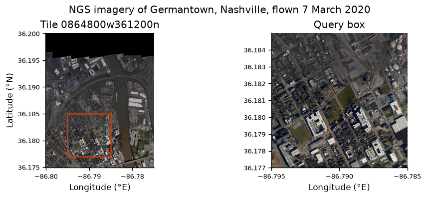

Saved plot from Post-event aerial imagery tiles

pixels = whole.reshape(-1, 3)
empty = (pixels.max(axis=1) == 0).mean()
print(f"Black, unimaged pixels in the overview: {empty:.0%}")
print(f"Full image decoded: {width * height * 3 / 1e9:.2f} GB of RGB")

Black, unimaged pixels in the overview: 17%
Full image decoded: 1.05 GB of RGB

The tile's top edge is beyond the flight, and JPEG tiles have no transparency band, so ground the flight did not cover is black. The Cumberland River runs through the tile, with Germantown's grid of streets west of it. At half a metre per pixel roofs and streets are clear; judging the damage to a roof needs the full image, four times finer, which Pillow can decode too at the cost of about a gigabyte of memory.

Pin and cite

verify checks the cached file against the lockfile's checksum. Keep the manifest and lockfile with your analysis; the citation below is what a methods section needs, and usdata cite dataset.yaml prints the same. NGS also publishes a citation per event, in its InPort record, which the dataset guide links.

assert verify(manifest) == []
for citation in cite_lockfile(manifest):
    print(citation.as_text())

noaa:emergency-response-imagery
  National Geodetic Survey, NOAA Emergency Response Imagery, accessed via usdata from https://registry.opendata.aws/noaa-eri
  homepage: https://storms.ngs.noaa.gov/
  license: US Government Work (public domain)
  terms: https://www.noaa.gov/information-technology/open-data-dissemination
  retrieved: 2026-09-29; 1 checksummed asset (58,670,760 bytes) pinned by usdata 0.33.0
  sources: 1

What was awkward

There is no reader. Pillow is enough to look at an overview, but analysis in map coordinates needs GDAL or rasterio, neither an extra, and Pillow cannot read the transparency masks or count the images in the file.
A bbox costs a header read for each folder, and it is refused outright for events whose files are numbered or oblique frames, such as Hurricane Wilma or Hurricane Matthew's oblique flights; there, name the tiled flights with collection.
The name is not quite the corner of the pixels: tiles extend 0.0001° past it, and some names round a second down, which is why footprints are widened and a tile beside the box can come along.
Time is a 30-hour UTC interval, because the folder gives a local date and nothing gives a time zone or an hour; start and end cannot select flights.
Tiles are large and grow: this one is 59 MB, and tiles flown since 2021 reach 1.7 GB. The dry run's byte count, and the 25 GB max_gb refusal, are worth reading before fetching a whole event.
Asset ids are whole bucket keys, since two folders can hold files of the same name, so the cached file name carries the event and flight with underscores for the slashes.

See the dataset guide for every event, file-naming scheme, and refusal.

Post-event aerial imagery tiles

At a glance

Quick start

Walkthrough