Monthly global 2 degree sea surface temperature since 1850

Saved results from a run against the live service; the notebook records when it ran and the checksums of what it read. Run it yourself.

The Extended Reconstructed Sea Surface Temperature is NOAA NCEI's monthly analysis of the global ocean's surface temperature on a 2 degree grid, rebuilt from ship, buoy, and Argo float observations back to January 1850. It is the record ENSO indices are computed from. NCEI publishes version 6, released in December 2025, as one NetCDF4 file per month, and each file holds two global grids: the temperature and its anomaly from the 1991-2020 climatology.

This walkthrough pulls the three months from May to July 2026, while an El Niño was building in the tropical Pacific, and computes the Niño 3.4 index from them. It needs usdata[netcdf] and matplotlib, and downloads three files of 168 kB each in a few seconds.

from datetime import UTC, datetime
from pathlib import Path

import matplotlib.pyplot as plt
import numpy as np
import xarray as xr
from matplotlib.patches import Rectangle

import usdata
from usdata import cite_lockfile, pull, verify

# One figure style for every usdata notebook, so previews look alike.
plt.rcParams.update(
    {
        "figure.figsize": (8, 4.5),
        "figure.dpi": 120,
        "axes.spines.top": False,
        "axes.spines.right": False,
        "axes.grid": True,
        "grid.alpha": 0.3,
        "font.size": 10,
    }
)
manifest = Path("dataset.yaml")
print("Executed (UTC):", datetime.now(UTC).isoformat(timespec="seconds"))
print(f"usdata {usdata.__version__}; xarray {xr.__version__}")

Executed (UTC): 2026-09-28T19:54:38+00:00
usdata 0.32.0; xarray 2026.7.0

Select

The manifest names a window and nothing else. ERSST files are whole global grids with no server-side subsetting, so there is no box, variable, or parameter to give; every calendar month the window touches is one file. May 1 to July 31 is May, June, and July. The newest month NCEI has published is preliminary until the next monthly update rewrites it, so the window stops a month short of it and the pins stay stable.

print(manifest.read_text())

name: ersst-el-nino-onset
sources:
  - dataset: noaa:ersst
    start: 2026-05-01
    end: 2026-07-31

What arrives

The first pull downloads three files and writes dataset.lock.json beside the manifest, pinning each checksum. The asset id is NCEI's filename, and the asset's time is the whole calendar month.

result = pull(manifest)
for item in result.fetched:
    month = item.asset.time.start
    print(f"{item.asset.id}  {item.provenance.size:,} bytes  {month:%B %Y}")
first = result.fetched[0].provenance
print("Source:", first.source_url)
print("Retrieved (UTC):", first.retrieved_at.isoformat(timespec="seconds"))
print("Checksum:", first.checksum)

ersst.v6.202605.nc  168,286 bytes  May 2026
ersst.v6.202606.nc  168,286 bytes  June 2026
ersst.v6.202607.nc  168,286 bytes  July 2026
Source: https://www.ncei.noaa.gov/data/sea-surface-temperature-extended-reconstructed/v6/access/ersst.v6.202605.nc
Retrieved (UTC): 2026-09-28T19:54:39+00:00
Checksum: sha256:51ce0020c969aea0aaff92184e7ba7e93f532a4ad378e734a9be1ab0d0731de8

Open

open() uses the netcdf extra and returns a loaded xarray Dataset. The grid is time × lev × lat × lon, one month at one nominal depth, with latitudes from 88°S to 88°N and longitudes from 0 to 358°E, both every 2 degrees at cell centres. sst is the monthly mean temperature and ssta its anomaly, both in degrees Celsius; land and sea ice are missing. The file stamps its time at mid-month.

months = [item.open().squeeze(["time", "lev"]) for item in result.fetched]
july = months[-1]
print("Variables:", {name: july[name].attrs["units"] for name in july.data_vars})
print("Grid:", dict(july.sizes), "· time", str(july.time.values)[:10])
print("Ocean cells:", int(july.sst.notnull().sum()), "of", july.sst.size)
print("Climatology:", july.attrs["climatology"])

Variables: {'sst': 'degree_C', 'ssta': 'degree_C'}
Grid: {'lat': 89, 'lon': 180} · time 2026-07-15
Ocean cells: 11074 of 16020
Climatology: Climatology is based on 1991-2020 SST of ERSSTv6.

The Niño 3.4 region is 5°S to 5°N and 170°W to 120°W, which is 190 to 240°E on this grid. Its mean anomaly, averaged over three consecutive months, is how ENSO strength is measured; five overlapping seasons at +0.5 °C or more make an El Niño.

def nino34(grid: xr.Dataset) -> float:
    """The mean anomaly over the Niño 3.4 box, 5° S-5° N and 190-240° E."""
    return float(grid.ssta.sel(lat=slice(-5, 5), lon=slice(190, 240)).mean())


for item, grid in zip(result.fetched, months, strict=True):
    print(f"{item.asset.time.start:%B %Y}: Niño 3.4 anomaly {nino34(grid):+.2f} °C")
print(f"May-July mean: {np.mean([nino34(grid) for grid in months]):+.2f} °C")

May 2026: Niño 3.4 anomaly +0.85 °C
June 2026: Niño 3.4 anomaly +1.44 °C
July 2026: Niño 3.4 anomaly +1.76 °C
May-July mean: +1.35 °C

The index rose by almost a degree in two months. CPC's traditional Oceanic Niño Index for May-July is +1.39 °C, also from ERSST v6, but on a 30-year base period centred on each era rather than one fixed 1991-2020 base. NOAA's official index since February 2026 is the Relative Oceanic Niño Index, which first subtracts the mean anomaly of the whole tropics, 20°N to 20°S; it is +0.97 °C for the same season, because the tropics are warm too.

A first look

fig, ax = plt.subplots(layout="constrained")
ax.set_facecolor("#e6e1d6")
mesh = ax.pcolormesh(
    july.lon, july.lat, july.ssta, cmap="RdBu_r", vmin=-4, vmax=4, shading="nearest"
)
ax.add_patch(Rectangle((189, -5), 52, 10, fill=False, edgecolor="black", linewidth=1.2))
ax.text(215, 7, "Niño 3.4", ha="center", fontsize=9)
ax.set_aspect("equal")
ax.grid(False)
ax.set_xlabel("Longitude (degrees east)")
ax.set_ylabel("Latitude (degrees north)")
ax.set_title("ERSST v6 sea surface temperature anomaly, July 2026")
fig.colorbar(mesh, ax=ax, label="Anomaly from 1991-2020 (°C)", shrink=0.8)
plt.show()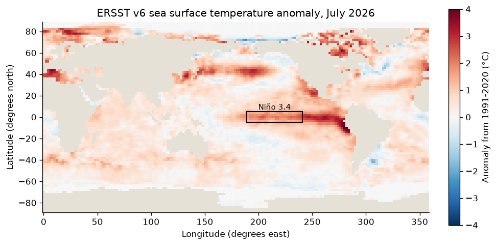

Saved plot from Monthly global 2 degree sea surface temperature since 1850

tropics = july.ssta.sel(lat=slice(-10, 10))
peak = tropics.where(tropics == tropics.max(), drop=True)
lat, lon = float(peak.lat[0]), float(peak.lon[0])
where = f"{abs(lat):.0f}° {'S' if lat < 0 else 'N'}, {360 - lon:.0f}° W"
print(f"Warmest tropical anomaly: {float(tropics.max()):+.2f} °C at {where}")
weights = np.cos(np.radians(july.lat))
print(f"Global area-weighted mean anomaly: {float(july.ssta.weighted(weights).mean()):+.2f} °C")

Warmest tropical anomaly: +4.79 °C at 10° S, 78° W
Global area-weighted mean anomaly: +0.55 °C

The warm tongue runs west along the equator from the coast of South America, strongest off Peru and Ecuador, where the anomaly reaches nearly 5 °C: the pattern of an El Niño growing from the east. The whole ocean averages half a degree above its 1991-2020 normal, so a basin-wide warm anomaly is not by itself an El Niño; the index is the tropical Pacific relative to that normal.

Pin and cite

verify checks the cached files against the lockfile's checksums. NCEI rewrites the newest month once, at the next monthly update, and rewrote every month from 2008 once in April 2026; a pin on a revised file reports it. Keep the manifest and lockfile with your results. The citation below is what a methods section needs, and usdata cite dataset.yaml prints the same.

assert verify(manifest) == []
for citation in cite_lockfile(manifest):
    print(citation.as_text())

noaa:ersst
  Huang, B., X. Yin, T. Boyer, C. Liu, M. Menne, Y. D. Rao, T. Smith, R. Vose, and H.-M. Zhang, 2025: Extended Reconstructed Sea Surface Temperature Version 6 (ERSSTv6): Part I. An Artificial Neural Network Approach. Journal of Climate, 38, 1105-1121, doi:10.1175/JCLI-D-23-0707.1
  homepage: https://www.ncei.noaa.gov/products/extended-reconstructed-sst
  license: US Government Work (public domain)
  terms: https://www.ncei.noaa.gov/products/extended-reconstructed-sst
  retrieved: 2026-09-28; 3 checksummed assets (504,858 bytes) pinned by usdata 0.32.0
  sources: 1

What was awkward

A Niño 3.4 value from these files is close to, not equal to, either index CPC publishes from them: ssta has one fixed base, 1991-2020, while ONI centres a base on each era and the official RONI also removes the tropical mean. Both indices are published only as CPC tables, not by NCEI.
The file stamps each month at its 15th while the asset's time is the whole month, and a Dataset opened from each file carries a one-step time and a one-level lev, so combining months starts with squeeze.
Longitudes run 0 to 360, so the Niño 3.4 box's western edge, 170°W, is 190 on this grid, and a map of the Pacific has to be drawn in those units.
The newest month is preliminary and nothing in the file or the listing says so; the monthly rewrite shows only in the directory's modified stamps.
Area weighting is left to the caller: a plain mean over the grid overweights high latitudes, where cells are smaller.

Monthly global 2 degree sea surface temperature since 1850

At a glance

Quick start

Walkthrough