NBM forecast guidance

Saved results from a run against the live service; the notebook records when it ran and the checksums of what it read. Run it yourself.

The National Blend of Models is NOAA's forecast guidance built from many models at once: it blends their output and corrects each for its known biases, so it is what a forecaster starts from rather than one model's run. NOAA issues it every hour to the anonymous noaa-nbm-grib2-pds bucket on AWS, and one GRIB2 file holds one run at one forecast hour for one region: the CONUS file is a 2.5 km grid of about 300 messages, 171 MB, with an index sidecar listing each message's byte offset.

This walkthrough fetches the 2 m temperature from the first four hours of the 20 UTC run on 6 May 2024 as byte ranges, maps the first hour across the country, and follows Oklahoma City into the evening. It needs usdata[grib] and matplotlib; the download is about 6 MB and the run takes about ten seconds.

from datetime import UTC, datetime, timedelta
from pathlib import Path

import matplotlib.pyplot as plt
import numpy as np
import pandas as pd
import xarray as xr

import usdata
from usdata import cite_lockfile, pull, verify

# One figure style for every usdata notebook, so previews look alike.
plt.rcParams.update(
    {
        "figure.figsize": (8, 4.5),
        "figure.dpi": 120,
        "axes.spines.top": False,
        "axes.spines.right": False,
        "axes.grid": True,
        "grid.alpha": 0.3,
        "font.size": 10,
    }
)
manifest = Path("dataset.yaml")
print("Executed (UTC):", datetime.now(UTC).isoformat(timespec="seconds"))
print(f"usdata {usdata.__version__}; xarray {xr.__version__}; numpy {np.__version__}")

Executed (UTC): 2026-09-24T06:14:35+00:00
usdata 0.26.0; xarray 2026.7.0; numpy 2.5.2

Select

The manifest names one run, four hours, and one field. The window selects runs by initialization time, so 20:00 to 20:00 UTC with cycle: 20 is the run started at 20 UTC on 6 May 2024. The blend has no hour 0: forecast_hour: [1, 2, 3, 4] is guidance valid at 21, 22, and 23 UTC and midnight. Later hours thin out to every 3 and then every 6 hours on a schedule that varies by cycle, and an hour a run does not publish is named after the listing.

messages names the field the way each file's .idx sidecar names it. NBM index lines carry a further text for ensemble statistics, so TMP:2 m above ground is the temperature itself and TMP:2 m above ground:1 hour fcst:ens std dev would be its spread. The source is named forecast so its files can be looked up by name.

print(manifest.read_text())

name: oklahoma-nbm-temperature
sources:
  - name: forecast
    dataset: noaa:nbm
    start: 2024-05-06T20:00:00Z
    end: 2024-05-06T20:00:00Z
    params:
      cycle: 20
      forecast_hour: [1, 2, 3, 4]
      messages: "TMP:2 m above ground"

What arrives

One small GRIB2 file per hour: the one named message, fetched as a byte range of that hour's CONUS object. The first pull writes dataset.lock.json beside the manifest, pinning each range and each object's ETag; a restore re-issues exactly those ranges, and a republished object is reported as drift. by_source returns the files in valid-time order.

result = pull(manifest)
files = result.by_source["forecast"]
pd.DataFrame(
    {
        "valid (UTC)": item.asset.time.start.strftime("%Y-%m-%d %H:%M"),
        "bytes": item.provenance.size,
        "object MB": round(item.provenance.object_size / 1e6, 1),
        "message": item.provenance.source_url.rsplit("=", 1)[1],
        "checksum": item.provenance.checksum[:19] + "...",
    }
    for item in files
)

	valid (UTC)	bytes	object MB	message	checksum
0	2024-05-06 21:00	1497346	171.1	279	sha256:505ca46ce4bd...
1	2024-05-06 22:00	1482290	167.9	273	sha256:afb8aab142b0...
2	2024-05-06 23:00	1466612	167.1	273	sha256:c19e57314393...
3	2024-05-07 00:00	1447461	173.3	281	sha256:a6724b446a6c...

first = files[0]
print("First file:", first.path.name)
print("Source:", first.provenance.source_url)
print("Retrieved (UTC):", first.provenance.retrieved_at.isoformat(timespec="seconds"))
print("Selector:", first.provenance.selectors[0])
print(f"Total: {sum(item.provenance.size for item in files) / 1e6:.1f} MB", end=" ")
print(f"of {sum(item.provenance.object_size for item in files) / 1e6:.0f} MB in the four objects")

First file: blend.20240506.t20z.core.f001.co.part-efd96aedf377.grib2
Source: s3://noaa-nbm-grib2-pds/blend.20240506/20/core/blend.t20z.core.f001.co.grib2#messages=279
Retrieved (UTC): 2026-09-24T06:14:36+00:00
Selector: TMP:2 m above ground
Total: 5.9 MB of 679 MB in the four objects

The temperature is message 279 in the first hour's file and 273 in the next two, so the position of a field is not fixed from hour to hour; naming it is what keeps the selection right.

Open

Each file is already a selection and opens without select. The variable is 2t, the ecCodes short name, in kelvin. The grid is Lambert conformal, 2345 × 1597 points about 2.5 km apart, so latitude and longitude are two-dimensional, and longitudes use the 0 to 360 convention. The run and valid times are in the variable's attributes.

fields = first.open()
temperature = fields["2t"]
print("Grid:", dict(fields.sizes), f"{fields.attrs['DxInMetres'] / 1000:.2f} km spacing")
print("Units:", temperature.attrs["units"], "·", temperature.attrs["name"])
print("Run:", temperature.attrs["reference_time"], "· valid:", temperature.attrs["valid_time"])

Grid: {'y': 1597, 'x': 2345} 2.54 km spacing
Units: K · 2 metre temperature
Run: 2024-05-06T20:00:00+00:00 · valid: 2024-05-06T21:00:00+00:00

A value at a place is the nearest grid point in two dimensions, after moving longitudes to −180 to 180. Every hour shares the grid, so the point is found once and read from each file in turn.

latitude = fields.latitude.values
longitude = np.where(
    fields.longitude.values > 180, fields.longitude.values - 360, fields.longitude.values
)
phi1, phi2 = np.radians(35.47), np.radians(latitude)  # Oklahoma City
dlat, dlon = phi2 - phi1, np.radians(longitude + 97.52)
h = np.sin(dlat / 2) ** 2 + np.cos(phi1) * np.cos(phi2) * np.sin(dlon / 2) ** 2
distance_km = 2 * 6371.0 * np.arcsin(np.sqrt(h))
y, x = np.unravel_index(distance_km.argmin(), distance_km.shape)
print(f"Nearest grid point: {latitude[y, x]:.3f} N {longitude[y, x]:.3f} E")
print(f"Distance from the city centre: {distance_km[y, x]:.1f} km")

central = timedelta(hours=-5)  # CDT
city = pd.DataFrame(
    {
        "valid (UTC)": item.asset.time.start.strftime("%H:%M"),
        "local (CDT)": (item.asset.time.start + central).strftime("%H:%M"),
        "forecast (°C)": round(float(item.open()["2t"][y, x]) - 273.15, 1),
    }
    for item in files
)
city

Nearest grid point: 35.475 N -97.509 E
Distance from the city centre: 1.2 km

	valid (UTC)	local (CDT)	forecast (°C)
0	21:00	16:00	26.2
1	22:00	17:00	26.3
2	23:00	18:00	26.1
3	00:00	19:00	25.8

A first look

The first hour's guidance, valid at 21 UTC (4 pm in Oklahoma), over the whole CONUS grid. The map plots the grid itself, which is already a Lambert conformal projection, so distances are in kilometres along the grid.

rows, cols = temperature.shape
spacing_km = fields.attrs["DxInMetres"] / 1000

fig, ax = plt.subplots(layout="constrained")
shaded = ax.imshow(
    temperature.values - 273.15,
    extent=(0, cols * spacing_km, 0, rows * spacing_km),
    cmap="RdYlBu_r",
    vmin=-5,
    vmax=40,
    interpolation="nearest",
)
ax.plot(
    x * spacing_km,
    (rows - 1 - y) * spacing_km,
    marker="*",
    markersize=11,
    color="white",
    markeredgecolor="black",
)
ax.annotate(
    "Oklahoma City",
    (x * spacing_km, (rows - 1 - y) * spacing_km),
    xytext=(8, 6),
    textcoords="offset points",
    fontsize=8,
)
ax.set_aspect("equal")
ax.grid(False)
ax.set(
    title="NBM 20 UTC run, 6 May 2024: 2 m temperature valid 21 UTC",
    xlabel="Distance east on the grid (km)",
    ylabel="Distance north on the grid (km)",
)
fig.colorbar(shaded, ax=ax, label="2 m temperature (°C)", shrink=0.8)
plt.show()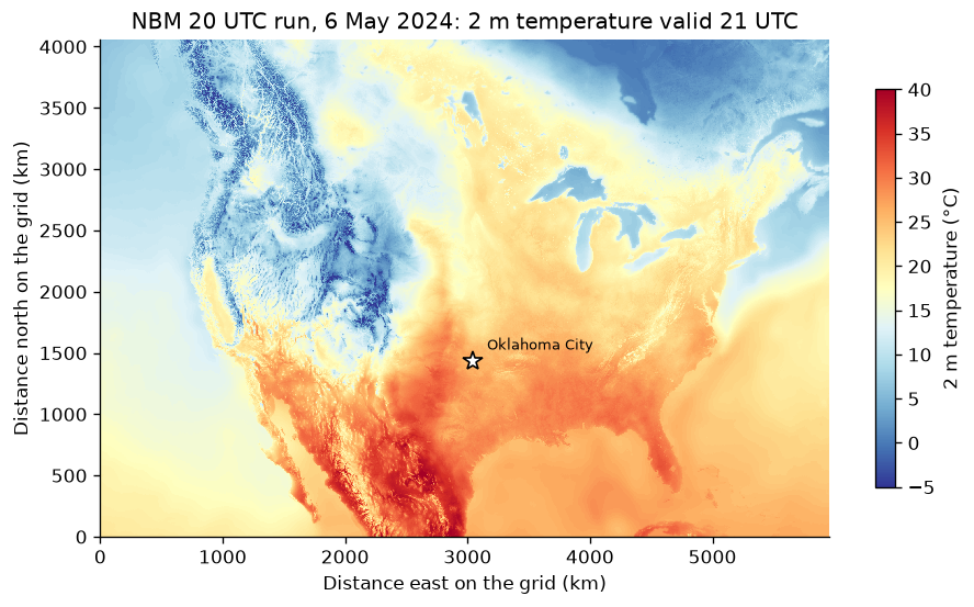

celsius = temperature.values - 273.15
hottest = np.unravel_index(int(np.nanargmax(celsius)), celsius.shape)
coldest = np.unravel_index(int(np.nanargmin(celsius)), celsius.shape)
for label, (i, j) in (("Warmest", hottest), ("Coldest", coldest)):
    print(f"{label}: {celsius[i, j]:.1f} °C at {latitude[i, j]:.2f} N {longitude[i, j]:.2f} E")
drop = city["forecast (°C)"].iloc[0] - city["forecast (°C)"].iloc[-1]
print(f"Oklahoma City cools {drop:.1f} °C from 21 UTC to midnight UTC")

Warmest: 41.1 °C at 27.10 N -101.57 E
Coldest: -14.1 °C at 51.37 N -125.26 E
Oklahoma City cools 0.4 °C from 21 UTC to midnight UTC

Cool air covered the Rockies and the northern High Plains while the southern Plains and the East sat in warm air, hottest in northern Mexico south of the Rio Grande. The coldest cell is a summit in the Coast Mountains of British Columbia, and the terrain of the West shows cell by cell at 2.5 km. Oklahoma City sat in the warm air and was expected to hold near 26 °C from 4 pm to 7 pm local time. The blend is guidance, not an observation: each value is the expected temperature at one 2.5 km cell.

Pin and cite

verify checks the cached bytes against the lockfile. Keep the manifest, lockfile, and cached bytes together; pull --update accepts new ranges after a republished object is reported as drift.

assert verify(manifest) == []
for citation in cite_lockfile(manifest):
    print(citation.as_text())

noaa:nbm
  NOAA National Blend of Models (NBM) was accessed on 2026-09-24 from https://registry.opendata.aws/noaa-nbm
  homepage: https://registry.opendata.aws/noaa-nbm/
  license: US Government Work (public domain)
  terms: https://www.noaa.gov/information-technology/open-data-dissemination
  retrieved: 2026-09-24; 4 checksummed assets (5,893,709 bytes) pinned by usdata 0.26.0
  sources: forecast

What was awkward

The CONUS grid stores every second row east to west (alternativeRowScanning), and the reader used to return those rows mirrored: the first map drawn for this notebook was a striped mirror image, and every value read at a point on half the rows came from the wrong column. The reader now reverses them; nothing in the file listing or the Dataset showed the problem short of drawing the field.
The 171 MB CONUS file makes messages the only sensible way in, but the index vocabulary has to be discovered from the sidecar itself: NBM lines carry a fourth field for ensemble spread and probability thresholds, and nothing in usdata info says which selectors a dataset's files hold. The guide's table is the substitute for a listing of the index.
Finding the grid point nearest a place takes a few lines of NumPy in every model walkthrough, after undoing the 0 to 360 longitude convention.
Temperature arrives in kelvin with the ecCodes short name 2t, which is not a valid Python identifier, so it is always read as fields["2t"].
The grib extra installs with pip alone on Linux, and on Windows through Python 3.13; macOS needs the ecCodes library from conda-forge or Homebrew first. The reader reference has the details.

NBM forecast guidance

At a glance

Quick start

Walkthrough