HRRR model output

Saved results from a run against the live service; the notebook records when it ran and the checksums of what it read. Run it yourself.

The High-Resolution Rapid Refresh is NOAA's 3 km forecast model for the contiguous United States, started every hour. NCEP publishes its GRIB2 output to the anonymous noaa-hrrr-bdp-pds bucket on AWS, and one file holds one run at one forecast hour: a whole CONUS grid of 170 fields in the surface set, about 150 MB.

This walkthrough pulls the 20 UTC analysis of 6 May 2024, the afternoon before a night of tornadoes in Oklahoma, reads surface CAPE, 0–3 km storm-relative helicity, and the land mask out of it, and maps where the two storm ingredients overlapped. It needs usdata[grib] and matplotlib; the download is 150 MB and the run takes about ten seconds.

from datetime import UTC, datetime
from pathlib import Path

import matplotlib.pyplot as plt
import numpy as np
import pandas as pd
import xarray as xr

import usdata
from usdata import cite_lockfile, pull, verify

# One figure style for every usdata notebook, so previews look alike.
plt.rcParams.update(
    {
        "figure.figsize": (8, 4.5),
        "figure.dpi": 120,
        "axes.spines.top": False,
        "axes.spines.right": False,
        "axes.grid": True,
        "grid.alpha": 0.3,
        "font.size": 10,
    }
)
manifest = Path("dataset.yaml")
print("Executed (UTC):", datetime.now(UTC).isoformat(timespec="seconds"))
print(f"usdata {usdata.__version__}; xarray {xr.__version__}; numpy {np.__version__}")

Executed (UTC): 2026-09-24T05:57:38+00:00
usdata 0.26.0; xarray 2026.7.0; numpy 2.5.2

Select

The manifest names one run and one hour. The window selects runs by initialization time, so 20:00 to 20:00 UTC with cycle: 20 is exactly the run started at 20 UTC on 6 May 2024. forecast_hour: 0 is that run's analysis: the model's own estimate of the atmosphere at initialization, a blend of the previous forecast with observations, rather than a projection forward. Forecast hour 1 would be a one-hour forecast valid at 21 UTC.

noaa:hrrr subsets in time only. This query downloads the whole surface file; naming GRIB2 messages with the messages parameter would fetch byte ranges of it instead, as the HRRR guide shows. usdata pull dataset.yaml --dry-run prints the size before anything is downloaded.

print(manifest.read_text())

name: oklahoma-hrrr-analysis
sources:
  - dataset: noaa:hrrr
    start: 2024-05-06T20:00:00Z
    end: 2024-05-06T20:00:00Z
    params:
      cycle: 20
      forecast_hour: 0

What arrives

One GRIB2 object from S3. The lockfile beside the manifest pins its name and SHA-256, so a pull with the lockfile present restores exactly these bytes. The provider notes describe no revision cycle for archived runs, so a checksum mismatch would mean a replaced or removed object.

result = pull(manifest)
(item,) = result.fetched
print("File:", item.path.name)
print(f"Bytes: {item.provenance.size} ({item.provenance.size / 1e6:.1f} MB)")
print("Source:", item.provenance.source_url)
print("Retrieved (UTC):", item.provenance.retrieved_at.isoformat(timespec="seconds"))
print("Checksum:", item.provenance.checksum)
print("Valid time:", item.asset.time.start.isoformat())

File: hrrr.20240506.t20z.wrfsfcf00.grib2
Bytes: 150114757 (150.1 MB)
Source: s3://noaa-hrrr-bdp-pds/hrrr.20240506/conus/hrrr.t20z.wrfsfcf00.grib2
Retrieved (UTC): 2026-09-24T05:57:42+00:00
Checksum: sha256:0f67cd6e1edd9d0876cb1a23459e9db59c892f7345e6a74b645b663302b7655c
Valid time: 2024-05-06T20:00:00+00:00

Open

A GRIB2 file is a stack of independent messages, one per field and level. item.inspect() lists them without decoding any values; each message carries the ecCodes keys that open_grib2(select=...) matches on.

messages = pd.DataFrame(
    message.model_dump(include={"short_name", "type_of_level", "level", "units"})
    for message in item.inspect().grib2.messages
)
print(len(messages), "messages;", (messages["short_name"] == "unknown").sum(), "named 'unknown'")
messages[messages["short_name"].isin(["cape", "hlcy", "lsm"])]

170 messages; 31 named 'unknown'

	short_name	type_of_level	level	units
104	cape	surface	0	J kg**-1
130	hlcy	heightAboveGroundLayer	3000	m2 s-2
131	hlcy	heightAboveGroundLayer	1000	m2 s-2
147	cape	pressureFromGroundLayer	18000	J kg**-1
151	cape	pressureFromGroundLayer	9000	J kg**-1
153	cape	pressureFromGroundLayer	25500	J kg**-1
157	cape	heightAboveGroundLayer	0	J kg**-1
164	lsm	surface	0	(0 - 1)

select matches every message that satisfies all of its keys, so three short names crossed with two level types decode five messages: the three wanted (surface CAPE, 0–3 km helicity, land mask) plus 0–1 km helicity and 0–3 km layer CAPE. Because the selection spans more than one level type, every variable is named shortName_typeOfLevel_level. Decoding is the slow step; five fields take a second or two.

The grid is Lambert conformal, 1799 × 1059 points 3 km apart, so latitude and longitude are two-dimensional coordinates, and longitudes use the 0 to 360 convention. Time is in each variable's attributes: valid_time is the initialization plus the forecast hour.

fields = item.open_grib2(
    select={
        "shortName": ["cape", "hlcy", "lsm"],
        "typeOfLevel": ["surface", "heightAboveGroundLayer"],
    }
)
pd.DataFrame(
    {
        "variable": name,
        "long_name": variable.attrs["name"],
        "units": variable.attrs["units"],
        "valid_time": variable.attrs["valid_time"],
        "shape": str(variable.shape),
    }
    for name, variable in fields.data_vars.items()
)

	variable	long_name	units	valid_time	shape
0	cape_surface_0	Convective available potential energy	J kg**-1	2024-05-06T20:00:00+00:00	(1059, 1799)
1	hlcy_heightAboveGroundLayer_3000	Storm relative helicity	m2 s-2	2024-05-06T20:00:00+00:00	(1059, 1799)
2	hlcy_heightAboveGroundLayer_1000	Storm relative helicity	m2 s-2	2024-05-06T20:00:00+00:00	(1059, 1799)
3	cape_heightAboveGroundLayer_0	Convective available potential energy	J kg**-1	2024-05-06T20:00:00+00:00	(1059, 1799)
4	lsm_surface_0	Land-sea mask	(0 - 1)	2024-05-06T20:00:00+00:00	(1059, 1799)

A value at a place means finding the nearest grid point in two dimensions, after moving longitudes to −180 to 180. The distance here is great-circle distance on a sphere, enough to pick a 3 km cell.

cape = fields["cape_surface_0"]
helicity = fields["hlcy_heightAboveGroundLayer_3000"]
latitude = fields.latitude.values
longitude = np.where(
    fields.longitude.values > 180, fields.longitude.values - 360, fields.longitude.values
)

place_lat, place_lon = 35.47, -97.52  # Oklahoma City
phi1, phi2 = np.radians(place_lat), np.radians(latitude)
dlat, dlon = phi2 - phi1, np.radians(longitude - place_lon)
haversine = np.sin(dlat / 2) ** 2 + np.cos(phi1) * np.cos(phi2) * np.sin(dlon / 2) ** 2
distance_km = 2 * 6371.0 * np.arcsin(np.sqrt(haversine))
y, x = np.unravel_index(distance_km.argmin(), distance_km.shape)
print(f"Nearest grid point to Oklahoma City: {latitude[y, x]:.3f} N {longitude[y, x]:.3f} E")
print(f"Distance from the city centre: {distance_km[y, x]:.1f} km")
print(f"Surface CAPE there: {float(cape[y, x]):.0f} J/kg")
print(f"0-3 km helicity there: {float(helicity[y, x]):.0f} m2/s2")

Nearest grid point to Oklahoma City: 35.477 N -97.506 E
Distance from the city centre: 1.5 km
Surface CAPE there: 3690 J/kg
0-3 km helicity there: 153 m2/s2

A first look

Surface CAPE is the energy available to a rising parcel; 0–3 km helicity measures the low-level wind shear a rotating storm can use. The map shades CAPE on the model's own grid, which is already a Lambert conformal projection, draws coastlines and lakes from the land mask, and hatches the cells where CAPE is at least 2000 J/kg and helicity at least 200 m²/s².

rows, cols = cape.shape
east_km = np.arange(cols) * 3.0
north_km = np.arange(rows)[::-1] * 3.0
overlap = (cape.values >= 2000) & (helicity.values >= 200)

fig, ax = plt.subplots(layout="constrained")
shaded = ax.imshow(
    np.ma.masked_less(cape.values, 100),
    extent=(0, cols * 3.0, 0, rows * 3.0),
    cmap="YlOrRd",
    vmin=0,
    vmax=4500,
    interpolation="nearest",
)
ax.contour(
    east_km, north_km, fields["lsm_surface_0"].values, levels=[0.5], colors="0.4", linewidths=0.5
)
ax.contourf(
    east_km, north_km, overlap.astype(float), levels=[0.5, 1.5], colors="none", hatches=["////"]
)
ax.plot(east_km[x], north_km[y], marker="*", markersize=11, color="cyan", markeredgecolor="black")
ax.annotate(
    "Oklahoma City",
    (east_km[x], north_km[y]),
    xytext=(8, 8),
    textcoords="offset points",
    fontsize=8,
)
ax.set_aspect("equal")
ax.grid(False)
ax.set(
    title=(
        "HRRR analysis valid 2024-05-06 20:00 UTC: surface CAPE\n"
        "hatched where CAPE ≥ 2000 J/kg and 0-3 km helicity ≥ 200 m²/s²"
    ),
    xlabel="Distance east on the grid (km)",
    ylabel="Distance north on the grid (km)",
)
fig.colorbar(shaded, ax=ax, label="Surface CAPE (J/kg)", shrink=0.8)
plt.show()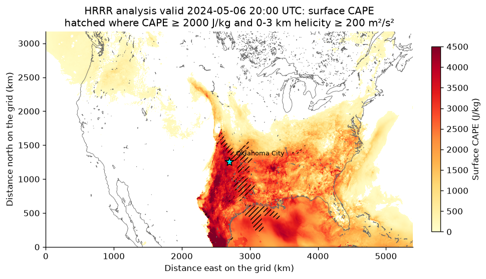

peak = np.unravel_index(int(np.nanargmax(cape.values)), cape.shape)
on_land = overlap & (fields["lsm_surface_0"].values >= 0.5)
print(f"Largest surface CAPE: {float(cape[peak]):.0f} J/kg")
print(f"  at {latitude[peak]:.2f} N {longitude[peak]:.2f} E")
print(f"Area with CAPE >= 2000 J/kg: {(cape.values >= 2000).sum() * 9:,} km2")
print(f"  and helicity >= 200 m2/s2 as well: {overlap.sum() * 9:,} km2")
print(f"  of which over land: {on_land.sum() * 9:,} km2")
near = on_land & (distance_km <= 300)
print(f"  of which within 300 km of Oklahoma City: {near.sum() * 9:,} km2")

Largest surface CAPE: 6420 J/kg
  at 28.58 N -101.11 E
Area with CAPE >= 2000 J/kg: 2,300,724 km2
  and helicity >= 200 m2/s2 as well: 271,188 km2
  of which over land: 171,360 km2
  of which within 300 km of Oklahoma City: 73,449 km2

Unstable air covered the southern and central United States east of a sharp western edge, the dryline, and the largest value in the domain sat just south of the Rio Grande in Mexico. Strong low-level shear overlapped it in a band along and east of that edge, from Kansas through Oklahoma into east Texas, and over the Gulf of Mexico. White areas hold less than 100 J/kg.

This is the afternoon environment, 8 hours 39 minutes before a tornado report in Oklahoma County at 04:39 UTC on 7 May, not the air that storm formed in; the run valid then is cycle: 4, forecast_hour: 0 on 7 May, a separate 150 MB file. CAPE and helicity are ingredients, not a tornado forecast, and each value is one 3 km cell of one model run.

The severe-weather case study reads that 04 UTC analysis for the same report, as two fields fetched by byte range, beside radar, lightning, and the report archives.

Pin and cite

verify checks the cached file against the lockfile's checksum. Keep the manifest, lockfile, and cached bytes together; public cloud retention is not a promise.

assert verify(manifest) == []
for citation in cite_lockfile(manifest):
    print(citation.as_text())

noaa:hrrr
  NOAA High-Resolution Rapid Refresh (HRRR) Model was accessed on 2026-09-16 from https://registry.opendata.aws/noaa-hrrr-pds
  homepage: https://registry.opendata.aws/noaa-hrrr-pds/
  license: US Government Work (public domain)
  terms: https://www.noaa.gov/information-technology/open-data-dissemination
  retrieved: 2026-09-16; 1 checksummed asset (150,114,757 bytes) pinned by usdata 0.18.0
  sources: 1

What was awkward

select crosses its keys: three short names and two level types decode five messages, and the two unwanted ones cost decode time and memory. Asking for exactly three fields that sit on different level types takes three open calls or a cross product like this one.
Units arrive as raw ecCodes strings, J kg**-1 and m**2 s**-2. Every plot label and sentence translates them by hand, and there is no documented canonical form to translate to.
31 of the 170 messages have the short name unknown, from HRRR's local parameter tables, and some (shortName, typeOfLevel, level) triples repeat. Those messages cannot be told apart by the keys the inventory shows; the guide says to select them by discipline, category, and parameter number.
Finding the grid point nearest a place is left to the caller, and every model walkthrough repeats the same few lines of NumPy, including undoing the 0 to 360 longitude convention first.
The projection arrives as raw ecCodes keys on Dataset.attrs (LaDInDegrees, Latin1InDegrees, DxInMetres, shapeOfTheEarth) with no CRS object, so drawing state borders or working in projected coordinates starts by rebuilding the projection from those keys. The map above plots the grid itself for that reason.
The retrieval URL is item.provenance.source_url while the asset's is item.asset.href: two names for the same idea on two objects usually used together.
The two dates in this notebook disagree. A pull that restores from the committed lockfile downloads the object again, so retrieved_at above is the day this notebook ran, while the citation says the file was accessed on the day the lockfile was first written. The citation is the one to quote, but nothing on the fetched item says so.
The grib extra installs with pip alone on Linux, and on Windows through Python 3.13; macOS needs the ecCodes library from conda-forge or Homebrew first. The reader reference has the details.

HRRR model output

At a glance

Quick start

Walkthrough

Select

What arrives

Open

A first look

Pin and cite

What was awkward

Used in these studies

For one Oklahoma tornado, do the two report archives agree on when and where it was, and what did radar, lightning, and the model analysis show at that place and time?

Reference