 usdata
One reported tornado, six national archives, one manifest, one lockfile. The notebook starts from the NCEI Storm Events annual archive for 2024, takes the time and position of event 1184052 out of it rather than assuming them, and then asks each of the other five sources what it recorded at that time and place: the Storm Prediction Center's own tornado file, the nearest KTLX Level II volume scan, five MRMS mid-level rotation grids, twenty minutes of GOES-16 lightning, and the HRRR analysis that ran last before the report.
The answer measures agreement between two publication paths for one storm survey, and what four remote-sensing and model products held within 25 km of the reported path start. It does not detect a tornado in any of those products, it does not establish that any of these quantities precede tornadoes in general, and it is one case. usdata only acquires the files; the analysis is pandas, numpy, and xarray.
It needs usdata[pandas,radar,netcdf,grib] and matplotlib; pyproj arrives
with the radar extra. The grib extra installs with pip alone on Linux and on
Windows through Python 3.13; macOS needs the ecCodes library from conda-forge or
Homebrew first (see the reader reference).
The manifest pins 84.9 MB, and a first run takes under a minute.
Show code
import gc
import subprocess
import sys
import time
from datetime import UTC, datetime, timedelta, timezone
from importlib.metadata import version
from pathlib import Path

import matplotlib.dates as mdates
import matplotlib.pyplot as plt
import numpy as np
import pandas as pd
from pyproj import Geod

from usdata import pull, verify

# One figure style for every usdata notebook, so previews look alike.
plt.rcParams.update(
    {
        "figure.figsize": (8, 4.5),
        "figure.dpi": 120,
        "axes.spines.top": False,
        "axes.spines.right": False,
        "axes.grid": True,
        "grid.alpha": 0.3,
        "font.size": 10,
    }
)
manifest = Path("dataset.yaml")
notebook_started = time.perf_counter()
pd.set_option("display.width", 130)
pd.set_option("display.max_columns", 20)
print("Executed (UTC):", datetime.now(UTC).isoformat(timespec="seconds"))
print(
    "; ".join(
        f"{name} {version(name)}"
        for name in ("usdata", "pandas", "numpy", "xarray", "xradar", "eccodes", "pyproj")
    )
)
Executed (UTC): 2026-09-24T05:58:12+00:00
usdata 0.26.0; pandas 3.0.6; numpy 2.5.2; xarray 2026.7.0; xradar 0.12.0; eccodes 2.48.0; pyproj 3.8.0
Data
Every file this notebook touches is declared once, in dataset.yaml, as six
named sources. The result is addressed by what each source is for rather than
by its position in a list: result.by_source["radar"] returns exactly the
assets that source resolved to, earliest first, result.one("reports") returns
the single file a one-file source resolved to, and the lockfile records the same
keys, so a restore rebuilds the grouping without re-resolving anything.
| Source | Dataset | What it pins | Why |
|---|---|---|---|
reports |
Storm Events | The whole 2024 annual details archive, selected by a 6 May 2024 window | The report's time, position, rating, and path |
spc |
SPC tornado reports | The whole 2024_torn.csv file |
The other national tornado archive, to check the report against |
radar |
NEXRAD Level II | Every KTLX volume scan between 04:34 and 04:46 UTC on 7 May 2024 | Reflectivity nearest the report time |
rotation |
MRMS | RotationTrackML30min_00.50 grids stamped 04:34 to 04:42 UTC |
Mid-level rotation merged from the radar network |
lightning |
GOES GLM | GOES-16 GLM files starting 04:29:00 to 04:48:59 UTC | Lightning ten minutes either side of the report |
environment |
HRRR | The CAPE and 0-3 km helicity messages of the 04 UTC analysis, surface file | The model environment last analysed before the report |
Report 1184052 is the same Oklahoma County tornado the smaller severe-weather studies use. They paste its time and position in as constants to stay small. This one puts the annual archive in the manifest instead, so every window below is measured against a number the notebook derived.
None of these services subsets on the server. Storm Events and the SPC file come
back as whole annual tables, MRMS and GOES-16 as whole CONUS or full-disk files,
and the HRRR run is one whole 3 km CONUS grid per field. The environment
source names the two GRIB2 messages it needs, so the fetch reads the object's
index and asks S3 for their byte ranges instead of the whole file: 1.8 MB of a
133 MB object. That is the client requesting part of a file, not a service
subsetting one, and the two fields still arrive on the full CONUS grid. Every
spatial narrowing below happens locally, after the download.
usdata pull dataset.yaml --dry-run prices the whole manifest before anything
is pulled: one line per asset, a subtotal per source, and the total on stderr.
Trimmed to the six subtotals and three of the seventy asset lines:
$ usdata pull dataset.yaml --dry-run
StormEvents_details-ftp_v1.0_d2024_c20260728.csv.gz	12693243	https://www.ncei.noaa.gov/pub/data/swdi/stormevents/csvfiles/StormEvents_details-ftp_v1.0_d2024_c20260728.csv.gz
reports (noaa:storm-events): 1 asset(s), 12693243 bytes
2024_torn.csv	?	https://www.spc.noaa.gov/wcm/data/2024_torn.csv
spc (noaa:spc-tornado-reports): 1 asset(s), at least 0 bytes; size unknown for 1 asset(s)
radar (noaa:nexrad-level2): 2 asset(s), 39708043 bytes
rotation (noaa:mrms): 5 asset(s), 926976 bytes
lightning (noaa:goes-glm): 60 asset(s), 29536150 bytes
hrrr.20240507.t04z.wrfsfcf00.part-13819cd0ccdf.grib2	1765823	s3://noaa-hrrr-bdp-pds/hrrr.20240507/conus/hrrr.t04z.wrfsfcf00.grib2#messages=105,131
environment (noaa:hrrr): 1 asset(s), 1765823 bytes
6 source(s), 70 asset(s), at least 84630235 bytes; size unknown for 1 asset(s) from spc; nothing downloaded
The HRRR line is the partial asset: a .part- digest of the resolved message
numbers in the id, the byte total of those two ranges, and the object it was cut
from with a #messages=105,131 fragment. The at least is the command
reporting that the SPC page publishes no size for 2024_torn.csv; its real
size appears only after the pull below.
Show code
geod = Geod(ellps="WGS84")
RADIUS_KM = 25.0
HALF_DEGREE = 0.5

print(manifest.read_text().strip())

started = time.perf_counter()
result = pull(manifest)
pull_seconds = time.perf_counter() - started

pinned = pd.DataFrame(
    {
        "source": key,
        "dataset": items[0].asset.dataset_id,
        "assets": len(items),
        "bytes": sum(item.provenance.size or 0 for item in items),
        "first_asset": items[0].asset.id,
    }
    for key, items in result.by_source.items()
)
total_bytes = int(pinned.bytes.sum())
print(f"\nPull seconds: {pull_seconds:.1f}")
print(f"Assets pinned: {len(result.fetched)}")
print(f"Total pinned bytes: {total_bytes:,} ({total_bytes / 1e6:.1f} MB)")
pinned
name: oklahoma-tornado-1184052
sources:
- name: reports
dataset: noaa:storm-events
start: 2024-05-06
end: 2024-05-06
- name: spc
dataset: noaa:spc-tornado-reports
start: 2024-01-01
end: 2024-12-31
- name: radar
dataset: noaa:nexrad-level2
start: 2024-05-07T04:34:00Z
end: 2024-05-07T04:46:00Z
params:
site: KTLX
- name: rotation
dataset: noaa:mrms
start: 2024-05-07T04:34:00Z
end: 2024-05-07T04:42:00Z
params:
product: RotationTrackML30min_00.50
- name: lightning
dataset: noaa:goes-glm
start: 2024-05-07T04:29:00Z
end: 2024-05-07T04:48:59Z
params:
satellite: 16
- name: environment
dataset: noaa:hrrr
start: 2024-05-07T04:00:00Z
end: 2024-05-07T04:00:00Z
params:
cycle: 4
forecast_hour: 0
file: sfc
messages: "CAPE:surface,HLCY:3000-0 m above ground"
Pull seconds: 13.2
Assets pinned: 70
Total pinned bytes: 84,860,329 (84.9 MB)
| source | dataset | assets | bytes | first_asset | |
|---|---|---|---|---|---|
| 0 | reports | noaa:storm-events | 1 | 12693243 | StormEvents_details-ftp_v1.0_d2024_c20260728.c... |
| 1 | spc | noaa:spc-tornado-reports | 1 | 230094 | 2024_torn.csv |
| 2 | radar | noaa:nexrad-level2 | 2 | 39708043 | KTLX20240507_043427_V06 |
| 3 | rotation | noaa:mrms | 5 | 926976 | MRMS_RotationTrackML30min_00.50_20240507-04340... |
| 4 | lightning | noaa:goes-glm | 60 | 29536150 | OR_GLM-L2-LCFA_G16_s20241280429000_e2024128042... |
| 5 | environment | noaa:hrrr | 1 | 1765823 | hrrr.20240507.t04z.wrfsfcf00.part-13819cd0ccdf... |
Which tornado, and exactly when and where
The 2024 annual details archive is one gzipped CSV of every Storm Events record for the year. It is 12.7 MB, and it is in the manifest so that the case can be selected from the archive rather than pasted in as constants: the report's identifier is the only thing this notebook assumes, and the time, the position, the rating, and the path come out of the file.
The timestamps in the file are local. CZ_TIMEZONE says which zone, and this
record says CST-6, a fixed offset with no daylight saving. The pandas reader
applies that rule itself: beside the untouched local columns the frame carries
BEGIN_UTC and END_UTC as UTC timestamps, and
attrs["usdata"]["derived"] states the rule it used and how many rows it could
not parse. The local evening of 6 May becomes the UTC early morning of 7 May.
Every other source in this notebook is stamped in UTC, so that one conversion is
what makes the rest of the comparison possible.
Show code
columns = [
    "EVENT_ID",
    "EVENT_TYPE",
    "STATE",
    "CZ_NAME",
    "CZ_TIMEZONE",
    "BEGIN_DATE_TIME",
    "END_DATE_TIME",
    "BEGIN_LAT",
    "BEGIN_LON",
    "END_LAT",
    "END_LON",
    "TOR_F_SCALE",
    "TOR_LENGTH",
    "TOR_WIDTH",
    "INJURIES_DIRECT",
    "DEATHS_DIRECT",
    "SOURCE",
]
reports_item = result.one("reports")
events = reports_item.open_csv(usecols=columns)
print("Records in the 2024 archive:", len(events))
for derived in events.attrs["usdata"]["derived"]:
    print(f"{derived['column']} from {derived['source']}: {derived['rule']}")
    print(f"  rows the rule could not parse: {derived['unparsed']}")

(report,) = events.loc[events.EVENT_ID.eq("1184052")].to_dict("records")
if pd.isna(report["BEGIN_UTC"]) or pd.isna(report["END_UTC"]):
    raise ValueError(f"No UTC time was derived from {report['CZ_TIMEZONE']!r}")
REPORT_UTC = report["BEGIN_UTC"].to_pydatetime()
END_UTC = report["END_UTC"].to_pydatetime()
LAT, LON = float(report["BEGIN_LAT"]), float(report["BEGIN_LON"])
END_LAT, END_LON = float(report["END_LAT"]), float(report["END_LON"])
_, _, straight_m = geod.inv(LON, LAT, END_LON, END_LAT)

for key, value in report.items():
    print(f"{key:18s} {value}")
print()
print("Report start, local:", report["BEGIN_DATE_TIME"], report["CZ_TIMEZONE"])
print("Report start, UTC:  ", REPORT_UTC.isoformat())
print("Report end, UTC:    ", END_UTC.isoformat())
print(f"Reported duration:   {(END_UTC - REPORT_UTC).total_seconds() / 60:.0f} minutes")
print(f"Start to end on the ground: {straight_m / 1000:.2f} km")
print(
    f"Reported path length: {report['TOR_LENGTH']} miles = {report['TOR_LENGTH'] * 1.609344:.2f} km"
)
print(f"Reported path width: {report['TOR_WIDTH']} yards = {report['TOR_WIDTH'] * 0.9144:.0f} m")

del events
gc.collect();
Records in the 2024 archive: 69801
BEGIN_UTC from BEGIN_DATE_TIME: local time parsed as %d-%b-%y %H:%M:%S, with years 50 to 99 read as 1950 to 1999, and shifted by the whole-hour UTC offset ending CZ_TIMEZONE (CST-6 is UTC-6, GST10 is UTC+10) or, for a bare label, by CST -6, EST -5, MST -7, PST -8, HST -10, CDT -5, EDT -4, or MDT -6; any other bare label is left unconverted
rows the rule could not parse: 0
END_UTC from END_DATE_TIME: local time parsed as %d-%b-%y %H:%M:%S, with years 50 to 99 read as 1950 to 1999, and shifted by the whole-hour UTC offset ending CZ_TIMEZONE (CST-6 is UTC-6, GST10 is UTC+10) or, for a bare label, by CST -6, EST -5, MST -7, PST -8, HST -10, CDT -5, EDT -4, or MDT -6; any other bare label is left unconverted
rows the rule could not parse: 0
EVENT_ID 1184052
STATE OKLAHOMA
EVENT_TYPE Tornado
CZ_NAME OKLAHOMA
BEGIN_DATE_TIME 06-MAY-24 22:39:00
CZ_TIMEZONE CST-6
END_DATE_TIME 06-MAY-24 22:42:00
INJURIES_DIRECT 0
DEATHS_DIRECT 0
SOURCE NWS Storm Survey
TOR_F_SCALE EF1
TOR_LENGTH 2.2
TOR_WIDTH 75.0
BEGIN_LAT 35.378
BEGIN_LON -97.543
END_LAT 35.397
END_LON -97.512
BEGIN_UTC 2024-05-07 04:39:00+00:00
END_UTC 2024-05-07 04:42:00+00:00
Report start, local: 06-MAY-24 22:39:00 CST-6
Report start, UTC: 2024-05-07T04:39:00+00:00
Report end, UTC: 2024-05-07T04:42:00+00:00
Reported duration: 3 minutes
Start to end on the ground: 3.52 km
Reported path length: 2.2 miles = 3.54 km
Reported path width: 75.0 yards = 69 m
Does the Storm Prediction Center's file say the same thing?
The SPC severe weather database is the other national tornado archive. Its 2024
file is 230 kB of plain CSV, one row per tornado when sg == 1. It has no
identifier in common with Storm Events, so the match has to be made on date,
position, and time.
The search below filters on the local calendar date derived in the previous
cell, keeps whole-track rows, and ranks every candidate in the country by
distance from the reported start point. SPC times are Central Standard Time for
every row, whatever zone the tornado was in, which the tz code of 3 states.
Nothing derives that clock for you, so this file is where the six-hour addition
is still written out by hand.
Show code
spc_item = result.one("spc")
spc = spc_item.open_csv(dtype={"stf": "string", "f1": "string"})
CST = timezone(timedelta(hours=-6))
local_date = REPORT_UTC.astimezone(CST).strftime("%Y-%m-%d")
print("SPC rows in 2024:", len(spc), "| whole-track rows:", int(spc.sg.eq(1).sum()))

candidates = spc.loc[spc.date.eq(local_date) & spc.sg.eq(1)].copy()
_, _, candidate_m = geod.inv(
    np.full(len(candidates), LON),
    np.full(len(candidates), LAT),
    candidates.slon.values,
    candidates.slat.values,
)
candidates["km_from_report"] = np.round(candidate_m / 1000, 2)
candidates = candidates.sort_values("km_from_report")
print(f"Whole-track tornadoes dated {local_date}: {len(candidates)}")
print(
    candidates.head(3)[
        ["om", "st", "time", "tz", "mag", "slat", "slon", "len", "wid", "km_from_report"]
    ].to_string(index=False)
)

spc_match = candidates.iloc[0]
if int(spc_match["tz"]) != 3:
    raise ValueError(f"Review the SPC timezone code before converting: {spc_match['tz']}")
spc_utc = (
    datetime.strptime(f"{spc_match['date']} {spc_match['time']}", "%Y-%m-%d %H:%M:%S")
    .replace(tzinfo=CST)
    .astimezone(UTC)
)
agreement = pd.DataFrame(
    [
        {
            "quantity": "start time (UTC)",
            "storm_events": REPORT_UTC.isoformat(),
            "spc": spc_utc.isoformat(),
        },
        {
            "quantity": "start latitude (degrees north)",
            "storm_events": LAT,
            "spc": float(spc_match["slat"]),
        },
        {
            "quantity": "start longitude (degrees east)",
            "storm_events": LON,
            "spc": float(spc_match["slon"]),
        },
        {
            "quantity": "rating",
            "storm_events": report["TOR_F_SCALE"],
            "spc": f"EF{int(spc_match['mag'])}",
        },
        {
            "quantity": "path length (miles)",
            "storm_events": report["TOR_LENGTH"],
            "spc": float(spc_match["len"]),
        },
        {
            "quantity": "path width (yards)",
            "storm_events": report["TOR_WIDTH"],
            "spc": float(spc_match["wid"]),
        },
    ]
)
print()
print(
    f"Separation: {spc_match['km_from_report']:.2f} km, "
    f"{(spc_utc - REPORT_UTC).total_seconds() / 60:.0f} minutes"
)
del spc, candidates
gc.collect()
agreement
SPC rows in 2024: 1873 | whole-track rows: 1791
Whole-track tornadoes dated 2024-05-06: 40
om st time tz mag slat slon len wid km_from_report
623971 OK 22:39:00 3 1 35.378 -97.543 2.2 75 0.00
623972 OK 22:46:00 3 1 35.427 -97.463 1.1 30 9.08
623964 OK 21:56:00 3 0 35.767 -97.016 2.2 50 64.38
Separation: 0.00 km, 0 minutes
| quantity | storm_events | spc | |
|---|---|---|---|
| 0 | start time (UTC) | 2024-05-07T04:39:00+00:00 | 2024-05-07T04:39:00+00:00 |
| 1 | start latitude (degrees north) | 35.378 | 35.378 |
| 2 | start longitude (degrees east) | -97.543 | -97.543 |
| 3 | rating | EF1 | EF1 |
| 4 | path length (miles) | 2.2 | 2.2 |
| 5 | path width (yards) | 75.0 | 75.0 |
The two agree exactly, and that is expected rather than reassuring: both publish the same NWS Storm Data entry, so the comparison shows that one survey survived two publication paths intact.
The radar volume nearest the report time
The manifest asks KTLX for every Level II volume scan between 04:34 and 04:46 UTC, which is two files of about 20 MB each, and the notebook picks the one whose scan start is nearest the report time derived above. Picking it here rather than in the manifest is the point: the choice follows from the archive, not from a timestamp typed into YAML.
A volume scan is not an instant. The lowest sweep is one rotation of the antenna, and its rays are stamped over about sixteen seconds. The gate positions below are computed from the radar's own location, each ray's azimuth, and the slant range projected onto the ground at the sweep's fixed elevation angle, with geodesic arithmetic on WGS84 rather than differences of degrees.
Show code
volumes = result.by_source["radar"]
for volume in volumes:
    offset = (volume.asset.time.start - REPORT_UTC).total_seconds()
    print(
        f"{volume.asset.id}  scan start {volume.asset.time.start:%H:%M:%S} UTC"
        f"  {offset:+.0f} s from the report"
    )

chosen = min(volumes, key=lambda item: abs((item.asset.time.start - REPORT_UTC).total_seconds()))
scan_offset = (chosen.asset.time.start - REPORT_UTC).total_seconds()
print("\nChosen:", chosen.asset.id)

radar = chosen.open_nexrad(sweep=0)
sweep = radar["sweep_0"].to_dataset()
radar_lat, radar_lon = float(radar.latitude), float(radar.longitude)
elevation = float(sweep.sweep_fixed_angle)
bearing, _, radar_m = geod.inv(radar_lon, radar_lat, LON, LAT)
effective_radius_km = 4 / 3 * 6371.0
range_km = radar_m / 1000
beam_km = (
    np.sqrt(
        range_km**2
        + effective_radius_km**2
        + 2 * range_km * effective_radius_km * np.sin(np.deg2rad(elevation))
    )
    - effective_radius_km
)
print(f"KTLX at {radar_lat:.4f} N {radar_lon:.4f} E, sweep elevation {elevation:.2f} degrees")
print(f"Report is {range_km:.2f} km from KTLX on a bearing of {bearing % 360:.1f} degrees")
print(f"Beam centre over the report: {beam_km:.2f} km above the radar (4/3 earth refraction)")
print("Sweep rays span", str(sweep.time.min().values), "to", str(sweep.time.max().values))

near = sweep.DBZH.sel(range=slice(None, 90_000))
azimuths = near.azimuth.values
ranges = near.range.values
order = np.argsort(azimuths)
azimuths, reflectivity = azimuths[order], near.values[order]


# Cell boundaries, so pcolormesh takes the mesh as given instead of inferring edges
# from coordinates that turn back on themselves as the antenna sweeps past north.
azimuth_step, range_step = float(np.diff(azimuths).mean()), float(np.diff(ranges).mean())
azimuth_edges = np.concatenate([azimuths - azimuth_step / 2, [azimuths[-1] + azimuth_step / 2]])
range_edges = np.concatenate([ranges - range_step / 2, [ranges[-1] + range_step / 2]])
ground = np.outer(np.ones_like(azimuth_edges), range_edges * np.cos(np.deg2rad(elevation)))
gate_lon, gate_lat, _ = geod.fwd(
    np.full(ground.shape, radar_lon),
    np.full(ground.shape, radar_lat),
    np.outer(azimuth_edges, np.ones_like(range_edges)),
    ground,
)
centre_ground = np.outer(np.ones_like(azimuths), ranges * np.cos(np.deg2rad(elevation)))
centre_lon, centre_lat, _ = geod.fwd(
    np.full(centre_ground.shape, radar_lon),
    np.full(centre_ground.shape, radar_lat),
    np.outer(azimuths, np.ones_like(ranges)),
    centre_ground,
)
_, _, gate_m = geod.inv(
    np.full(centre_ground.shape, LON), np.full(centre_ground.shape, LAT), centre_lon, centre_lat
)
gate_km = gate_m / 1000
in_radius = gate_km <= RADIUS_KM
print(
    f"\nUnits: {near.attrs['units']}; gates kept: {reflectivity.size}, "
    f"within {RADIUS_KM:.0f} km of the report: {int(in_radius.sum())}"
)
max_dbz = float(np.nanmax(np.where(in_radius, reflectivity, np.nan)))
print(f"Maximum reflectivity within {RADIUS_KM:.0f} km: {max_dbz:.1f} dBZ")
del radar, sweep, near
gc.collect();
KTLX20240507_043427_V06 scan start 04:34:27 UTC -273 s from the report
KTLX20240507_044053_V06 scan start 04:40:53 UTC +113 s from the report
Chosen: KTLX20240507_044053_V06
KTLX at 35.3334 N -97.2778 E, sweep elevation 0.48 degrees
Report is 24.61 km from KTLX on a bearing of 281.7 degrees
Beam centre over the report: 0.24 km above the radar (4/3 earth refraction)
Sweep rays span 2024-05-07T04:40:53.536000000 to 2024-05-07T04:41:09.636999936

Units: dBZ; gates kept: 253440, within 25 km of the report: 43672
Maximum reflectivity within 25 km: 62.5 dBZ
The chosen scan begins shortly after the report and its lowest sweep spans about sixteen seconds, so it is near the report rather than simultaneous with it.
Mid-level rotation around the report
MRMS RotationTrackML30min_00.50 merges azimuthal shear from every radar in the
network over the 3 to 6 km layer and writes a CONUS grid every two minutes. Each
value is the largest shear seen in the thirty minutes ending at the file stamp,
so the grid stamped 04:42 covers 04:12 to 04:42 and is the first one whose window
contains the whole reported tornado.
The files carry no units of their own. The registry entry supplies them, and
dataset.attrs["usdata"]["registry_attrs"] lists exactly which attributes were
filled in that way, so a value read out of the file can be printed with a unit
without consulting a web page. The decoded variable is called
RotationTrackML30min, without the _00.50 suffix the manifest must use.
The grids are 7,000 by 14,000 points and about 0.39 GB once decoded, so each one is cropped to a half-degree box around the report and released before the next is opened. Values are quantized to whole units of 0.001 per second, so several cells can tie at a box maximum; the table reports the tie count and averages the tied positions instead of letting array order choose one.
Show code
rotation_rows = []
rotation_field = None
for grid_item in result.by_source["rotation"]:
    grid = grid_item.open()
    (variable,) = grid.data_vars
    latitudes = grid.latitude.values
    longitudes = grid.longitude.values - 360.0
    rows = np.flatnonzero(np.abs(latitudes - LAT) <= HALF_DEGREE)
    cols = np.flatnonzero(np.abs(longitudes - LON) <= HALF_DEGREE)
    box_lat = latitudes[rows.min() : rows.max() + 1]
    box_lon = longitudes[cols.min() : cols.max() + 1]
    box = grid[variable].values[rows.min() : rows.max() + 1, cols.min() : cols.max() + 1]
    mesh_lon, mesh_lat = np.meshgrid(box_lon, box_lat)
    _, _, cell_m = geod.inv(np.full(box.shape, LON), np.full(box.shape, LAT), mesh_lon, mesh_lat)
    cell_km = cell_m / 1000
    circle = cell_km <= RADIUS_KM
    peak = float(np.max(np.where(circle, box, -np.inf)))
    tied = np.argwhere(circle & (box == peak))
    peak_lat = float(box_lat[tied[:, 0]].mean())
    peak_lon = float(box_lon[tied[:, 1]].mean())
    _, _, peak_m = geod.inv(LON, LAT, peak_lon, peak_lat)
    stamp = grid_item.asset.time.start
    rotation_rows.append(
        {
            "window_utc": f"{(stamp - timedelta(minutes=30)):%H:%M} to {stamp:%H:%M}",
            "peak_in_25km": peak,
            "tied_cells": len(tied),
            "peak_lat": round(peak_lat, 3),
            "peak_lon": round(peak_lon, 3),
            "km_from_report": round(peak_m / 1000, 1),
            "at_report_cell": float(box[np.unravel_index(int(cell_km.argmin()), cell_km.shape)]),
        }
    )
    if stamp.minute == 42:
        rotation_field = (box_lat.copy(), box_lon.copy(), box.copy())
        rotation_units = grid[variable].attrs["units"]
        rotation_name = grid[variable].attrs["long_name"]
        registry_attrs = grid.attrs["usdata"]["registry_attrs"]
        rotation_variable = variable
    del grid, box, cell_km, circle, mesh_lon, mesh_lat
    gc.collect()

rotation = pd.DataFrame(rotation_rows)
print("Decoded variable:", rotation_variable)
print("long_name:", rotation_name)
print("units:", rotation_units)
print("Filled from the registry entry:", registry_attrs)
rotation
Decoded variable: RotationTrackML30min
long_name: 30-minute maximum mid-level azimuthal shear
units: 0.001 s-1
Filled from the registry entry: [{'variable': 'RotationTrackML30min', 'attribute': 'units'}, {'variable': 'RotationTrackML30min', 'attribute': 'long_name'}]
| window_utc | peak_in_25km | tied_cells | peak_lat | peak_lon | km_from_report | at_report_cell | |
|---|---|---|---|---|---|---|---|
| 0 | 04:04 to 04:34 | 13.0 | 4 | 35.349 | -97.754 | 19.4 | 0.0 |
| 1 | 04:06 to 04:36 | 13.0 | 7 | 35.337 | -97.715 | 16.3 | 3.0 |
| 2 | 04:08 to 04:38 | 13.0 | 7 | 35.337 | -97.715 | 16.3 | 3.0 |
| 3 | 04:10 to 04:40 | 13.0 | 7 | 35.337 | -97.715 | 16.3 | 3.0 |
| 4 | 04:12 to 04:42 | 18.0 | 1 | 35.377 | -97.543 | 0.1 | 18.0 |
Lightning in the twenty minutes around the report
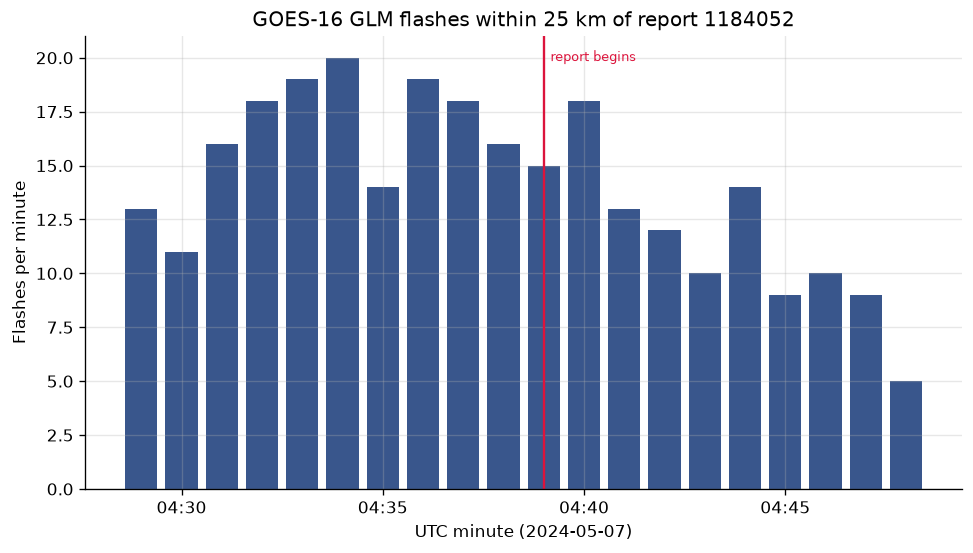
GOES-16's Geostationary Lightning Mapper writes one file every twenty seconds covering its whole field of view. The manifest pins the sixty files whose start times fall between 04:29:00 and 04:48:59 UTC, ten minutes either side of the report, about 30 MB in total.
Flash positions, times, and identifiers arrive as xarray coordinates rather than
data variables, so they have to be promoted with reset_coords() before
to_dataframe() will keep them. A flash centroid is an energy-weighted
cloud-top position, not a ground strike, and one flash can span several counties
and still count once. The series below is binned on each flash's first
constituent event, which can fall a fraction of a second before the start of the
file it was written into.
Show code
glm_columns = [
    "flash_lat",
    "flash_lon",
    "flash_time_offset_of_first_event",
    "flash_quality_flag",
]
frames = []
for glm_item in result.by_source["lightning"]:
    detections = glm_item.open()
    frames.append(detections[glm_columns].reset_coords()[glm_columns].to_dataframe())
    detections.close()
    del detections
flashes = pd.concat(frames, ignore_index=True)
_, _, flash_m = geod.inv(
    np.full(len(flashes), LON),
    np.full(len(flashes), LAT),
    flashes.flash_lon.values,
    flashes.flash_lat.values,
)
flashes["km_from_report"] = flash_m / 1000

nearby = flashes.loc[flashes.km_from_report <= RADIUS_KM]
box_flashes = flashes.loc[
    flashes.flash_lat.between(LAT - HALF_DEGREE, LAT + HALF_DEGREE)
    & flashes.flash_lon.between(LON - HALF_DEGREE, LON + HALF_DEGREE)
]
print(f"Flashes in the whole field of view, 04:29 to 04:49 UTC: {len(flashes):,}")
print(f"Within the half-degree box: {len(box_flashes):,}")
print(f"Within {RADIUS_KM:.0f} km of the report: {len(nearby):,}")
print("Quality flags among those:", nearby.flash_quality_flag.value_counts().to_dict())

per_minute = nearby.flash_time_offset_of_first_event.dt.floor("min").value_counts().sort_index()
mark = pd.Timestamp(REPORT_UTC).tz_localize(None)
before, after = per_minute.loc[per_minute.index < mark], per_minute.loc[per_minute.index >= mark]
print(f"\nMean rate in the ten minutes before the report: {before.mean():.1f} flashes per minute")
print(f"Mean rate from the report onward:                 {after.mean():.1f} flashes per minute")
print(f"Busiest minute: {per_minute.idxmax():%H:%M} UTC with {per_minute.max()} flashes")

fig, ax = plt.subplots(layout="constrained")
ax.bar(per_minute.index, per_minute.values, width=pd.Timedelta(minutes=0.8), color="#39568c")
ax.axvline(mark, color="crimson", linewidth=1.4)
ax.annotate(
    "report begins",
    xy=(mark, per_minute.max()),
    xytext=(4, -2),
    textcoords="offset points",
    color="crimson",
    fontsize=8,
)
ax.set(
    xlabel="UTC minute (2024-05-07)",
    ylabel="Flashes per minute",
    title=f"GOES-16 GLM flashes within {RADIUS_KM:.0f} km of report 1184052",
)
ax.xaxis.set_major_formatter(mdates.DateFormatter("%H:%M"))
plt.show()
plt.close(fig)
del frames, flashes
gc.collect();
Flashes in the whole field of view, 04:29 to 04:49 UTC: 14,897
Within the half-degree box: 479
Within 25 km of the report: 279
Quality flags among those: {0.0: 279}
Mean rate in the ten minutes before the report: 16.4 flashes per minute
Mean rate from the report onward: 11.5 flashes per minute
Busiest minute: 04:34 UTC with 20 flashes
The model environment thirty-nine minutes earlier
HRRR runs every hour, and forecast hour 0 of a run is its analysis, the model's
own estimate of the atmosphere at initialization rather than a projection
forward. The last analysis before a 04:39 UTC report is the run initialized at
04:00 UTC, so the manifest pins cycle: 4, forecast_hour: 0, the surface file:
one 133 MB object holding 170 GRIB2 messages, two of which this notebook reads.
The source names those two in messages, spelled the way the object's .idx
sidecar spells them, CAPE:surface and HLCY:3000-0 m above ground, rather than
the way the reader's select does. The fetch resolves them through the index and
asks for their byte ranges, so the asset is 1,765,823 bytes instead of
133,253,838, its id carries a .part- digest of the message numbers, and the
lockfile pins the ranges and the object's ETag.
inspect() reports what arrived, as data: two messages with their shortName,
typeOfLevel, level, units, and shape. Because the fetch already selected,
open() takes no select here. The two messages sit on two types of level, so
both variables are named shortName_typeOfLevel_level, and
attrs["usdata"]["messages"] maps each name back to its message, which is where
the cell below reads the two names from instead of assuming them.
Show code
environment = result.one("environment")
summary = environment.inspect()
inventory = pd.DataFrame(
    {
        "shortName": message.short_name,
        "typeOfLevel": message.type_of_level,
        "level": message.level,
        "units": message.units,
        "name": message.name,
    }
    for message in summary.grib2.messages
)
print(
    f"{summary.asset_id}: {summary.format.value}, {summary.size:,} bytes, {len(inventory)} messages"
)
print("\nEvery message the partial fetch brought back:")
print(inventory.to_string())

started = time.perf_counter()
fields = environment.open()
messages = fields.attrs["usdata"]["messages"]
cape_name = next(name for name, message in messages.items() if message["shortName"] == "cape")
helicity_name = next(name for name, message in messages.items() if message["shortName"] == "hlcy")
analysis_utc = environment.asset.time.start
lead = REPORT_UTC - analysis_utc
print(f"\nDecode seconds: {time.perf_counter() - started:.1f}")
print("Variable names, from attrs['usdata']['messages']:")
for name, message in messages.items():
    print(f"  {name}: message {message['file_index']} of the fetched file, step {message['step']}")
print("Analysis valid:", analysis_utc.isoformat())
print(f"Report follows the analysis by {lead} ({lead.total_seconds() / 60:.0f} minutes)")

latitudes = fields.latitude.values
stored = fields.longitude.values
longitudes = np.where(stored > 180, stored - 360, stored)
rows, cols = np.where((np.abs(latitudes - LAT) <= 0.6) & (np.abs(longitudes - LON) <= 0.75))
window = (slice(rows.min(), rows.max() + 1), slice(cols.min(), cols.max() + 1))
model_lat, model_lon = latitudes[window], longitudes[window]
_, _, model_m = geod.inv(
    np.full(model_lat.shape, LON), np.full(model_lat.shape, LAT), model_lon, model_lat
)
model_km = model_m / 1000
nearest = np.unravel_index(int(model_km.argmin()), model_km.shape)
circle = model_km <= RADIUS_KM
print(
    f"Nearest grid cell: {model_lat[nearest]:.4f} N {model_lon[nearest]:.4f} E, "
    f"{model_km[nearest]:.2f} km from the report (grid spacing is 3 km); "
    f"{int(circle.sum())} cells within {RADIUS_KM:.0f} km"
)

environment_rows = []
for label, variable in (
    ("surface CAPE", cape_name),
    ("0-3 km storm-relative helicity", helicity_name),
):
    values = fields[variable].values[window]
    environment_rows.append(
        {
            "field": label,
            "variable": variable,
            "units": fields[variable].attrs["units"],
            "at_report_cell": round(float(values[nearest]), 1),
            "median_in_25km": round(float(np.median(values[circle])), 1),
            "max_in_25km": round(float(values[circle].max()), 1),
        }
    )
del fields
gc.collect()
pd.DataFrame(environment_rows)
hrrr.20240507.t04z.wrfsfcf00.part-13819cd0ccdf.grib2: grib2, 1,765,823 bytes, 2 messages
Every message the partial fetch brought back:
shortName typeOfLevel level units name
0 cape surface 0 J kg**-1 Convective available potential energy
1 hlcy heightAboveGroundLayer 3000 m**2 s**-2 Storm relative helicity
Decode seconds: 0.4
Variable names, from attrs['usdata']['messages']:
  cape_surface_0: message 0 of the fetched file, step 0
  hlcy_heightAboveGroundLayer_3000: message 1 of the fetched file, step 0
Analysis valid: 2024-05-07T04:00:00+00:00
Report follows the analysis by 0:39:00 (39 minutes)
Nearest grid cell: 35.3693 N -97.5388 E, 1.04 km from the report (grid spacing is 3 km); 221 cells within 25 km
| field | variable | units | at_report_cell | median_in_25km | max_in_25km | |
|---|---|---|---|---|---|---|
| 0 | surface CAPE | cape_surface_0 | J kg**-1 | 3320.0 | 3530.0 | 5010.0 |
| 1 | 0-3 km storm-relative helicity | hlcy_heightAboveGroundLayer_3000 | m**2 s**-2 | 379.0 | 409.0 | 658.0 |
One picture of what the radars saw
The left panel is the chosen KTLX sweep, cropped to the half-degree box, with the reported path drawn on it and every GLM flash centroid from the twenty-minute window shown as a white dot. The right panel is the MRMS grid stamped 04:42, the thirty-minute mid-level shear maximum whose window contains the report.
The two panels are different quantities on different grids at different times. Reflectivity is one instant from one radar at a beam height of about a quarter of a kilometre over the report; the shear field is a half-hour maximum merged from the whole network in the 3 to 6 km layer. They are drawn side by side because they share a map, not because they measure the same thing.
Show code
box_lat, box_lon, box_values = rotation_field
fig, axes = plt.subplots(1, 2, layout="constrained")

ax = axes[0]
mesh = ax.pcolormesh(
    gate_lon, gate_lat, reflectivity, cmap="turbo", shading="flat", vmin=-10, vmax=65
)
ax.scatter(
    box_flashes.flash_lon,
    box_flashes.flash_lat,
    s=4,
    c="white",
    alpha=0.55,
    linewidths=0,
    label="GLM flash centroid",
)
ax.plot([LON, END_LON], [LAT, END_LAT], color="black", linewidth=1.6, label="Reported path")
ax.scatter(
    LON, LAT, marker="*", s=200, c="magenta", edgecolors="black", zorder=5, label="Report start"
)
ax.scatter(radar_lon, radar_lat, marker="^", s=70, c="black", zorder=5, label="KTLX")
ax.legend(loc="lower left", fontsize=6.5, facecolor="0.8")
ax.grid(False)
ax.set(
    xlim=(LON - HALF_DEGREE, LON + HALF_DEGREE),
    ylim=(LAT - HALF_DEGREE, LAT + HALF_DEGREE),
    xlabel="Longitude (degrees east)",
    ylabel="Latitude (degrees north)",
    title=f"KTLX {elevation:.2f}° sweep, {chosen.asset.time.start:%H:%M:%S} UTC",
    aspect=1 / np.cos(np.deg2rad(LAT)),
)
fig.colorbar(mesh, ax=ax, label="Reflectivity (dBZ)", shrink=0.8)

ax = axes[1]
mesh = ax.pcolormesh(box_lon, box_lat, box_values, cmap="magma", shading="nearest", vmin=0, vmax=20)
ax.scatter(LON, LAT, marker="*", s=200, c="cyan", edgecolors="black", zorder=5)
ax.plot([LON, END_LON], [LAT, END_LAT], color="cyan", linewidth=1.2)
ax.grid(False)
ax.set(
    xlim=(LON - HALF_DEGREE, LON + HALF_DEGREE),
    ylim=(LAT - HALF_DEGREE, LAT + HALF_DEGREE),
    xlabel="Longitude (degrees east)",
    title="MRMS mid-level shear, 04:12 to 04:42 UTC",
    aspect=1 / np.cos(np.deg2rad(LAT)),
)
fig.colorbar(mesh, ax=ax, label=f"Azimuthal shear ({rotation_units})", shrink=0.8)
for ax in axes:
    ax.title.set_fontsize(9)
fig.suptitle("Tornado report 1184052, Oklahoma County, 7 May 2024")
plt.show()
plt.close(fig)
del gate_lon, gate_lat, centre_lon, centre_lat, reflectivity, gate_km, in_radius
gc.collect();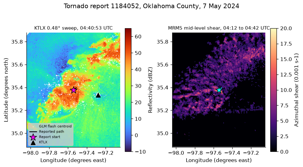
The reported path runs through high reflectivity on the KTLX sweep, and the strongest mid-level shear in the half-hour window sits on the reported start point.
What the six sources add up to
One row per source, each number carried down from the cell that produced it.
Show code
answer = pd.DataFrame(
    [
        {
            "source": "reports",
            "dataset": "noaa:storm-events",
            "what it gave": "event 1184052: EF1, 04:39:00 to 04:42:00 UTC, "
            f"{LAT} N {LON} E, {report['TOR_LENGTH']} mi by {report['TOR_WIDTH']} yd, "
            f"{report['INJURIES_DIRECT']} injuries",
        },
        {
            "source": "spc",
            "dataset": "noaa:spc-tornado-reports",
            "what it gave": f"tornado {int(spc_match['om'])}: same start time, "
            f"{spc_match['km_from_report']:.2f} km from the same point, "
            f"EF{int(spc_match['mag'])}, {spc_match['len']} mi by {int(spc_match['wid'])} yd",
        },
        {
            "source": "radar",
            "dataset": "noaa:nexrad-level2",
            "what it gave": f"KTLX sweep starting {scan_offset:+.0f} s from the report, "
            f"beam {beam_km:.2f} km up, "
            f"{max_dbz:.1f} dBZ maximum within {RADIUS_KM:.0f} km",
        },
        {
            "source": "rotation",
            "dataset": "noaa:mrms",
            "what it gave": f"mid-level shear peak {rotation.peak_in_25km.iloc[-1]:.0f} "
            f"({rotation_units}) in the 04:12 to 04:42 window, "
            f"{rotation.km_from_report.iloc[-1]:.1f} km from the reported start",
        },
        {
            "source": "lightning",
            "dataset": "noaa:goes-glm",
            "what it gave": f"{len(nearby):,} flashes within {RADIUS_KM:.0f} km in 20 minutes, "
            f"{before.mean():.1f} per minute before the report and {after.mean():.1f} after",
        },
        {
            "source": "environment",
            "dataset": "noaa:hrrr",
            "what it gave": f"04:00 UTC analysis, {lead.total_seconds() / 60:.0f} minutes early: "
            f"{environment_rows[0]['at_report_cell']:.0f} J/kg surface CAPE and "
            f"{environment_rows[1]['at_report_cell']:.0f} m2/s2 0-3 km helicity at the report cell",
        },
    ]
)
pd.set_option("display.max_colwidth", 150)
answer| source | dataset | what it gave | |
|---|---|---|---|
| 0 | reports | noaa:storm-events | event 1184052: EF1, 04:39:00 to 04:42:00 UTC, 35.378 N -97.543 E, 2.2 mi by 75.0 yd, 0 injuries |
| 1 | spc | noaa:spc-tornado-reports | tornado 623971: same start time, 0.00 km from the same point, EF1, 2.2 mi by 75 yd |
| 2 | radar | noaa:nexrad-level2 | KTLX sweep starting +113 s from the report, beam 0.24 km up, 62.5 dBZ maximum within 25 km |
| 3 | rotation | noaa:mrms | mid-level shear peak 18 (0.001 s-1) in the 04:12 to 04:42 window, 0.1 km from the reported start |
| 4 | lightning | noaa:goes-glm | 279 flashes within 25 km in 20 minutes, 16.4 per minute before the report and 11.5 after |
| 5 | environment | noaa:hrrr | 04:00 UTC analysis, 39 minutes early: 3320 J/kg surface CAPE and 379 m2/s2 0-3 km helicity at the report cell |
What the answer does not show
- The two archives are not two independent observations. Storm Events and the SPC file both derive from the same NWS Storm Data entry for this tornado, which is why their start time, coordinates, rating, path length, and path width match exactly rather than approximately. Agreement here means the two publication paths carried one survey faithfully. It is not corroboration. The two databases share no identifier, so the match is made on local date, whole-track rows, and distance from the derived point.
- Times come from three different clocks. Storm Events timestamps are local,
labelled by a
CZ_TIMEZONEstring,CST-6here. SPC rows are Central Standard Time for every tornado in the country, whatever zone it was in. Everything else is UTC. - None of the remote sensing detects a tornado. Reflectivity, azimuthal shear, and flash counts describe a storm. The tornado in this notebook exists only because a survey crew wrote it down; every other number is context around a point that the survey supplied.
- The radar volume is chosen, not pinned. The manifest resolves to two volume scans and the notebook keeps the one nearest the derived report time, which starts after the report rather than at it.
- The MRMS peak in the report's own cell is a coincidence of resolution, not a measurement of the vortex. The grid is 0.005 degrees, values are quantized to whole units of 0.001 per second, and each one is a maximum over the preceding thirty minutes, so a peak landing next to the reported start point is a half-hour accumulation nearest that cell, not shear observed at 04:39.
- Mid-level shear is not low-level rotation. This product samples the 3 to 6 km layer, well above a tornado, and its magnitude depends on how far each contributing radar was and at what angle it looked.
- The 25 km radius is an analysis choice. It is written into the notebook, not supplied by the package, and a different radius moves every maximum in the tables.
- The lightning rate is one storm's. Twenty minutes of one storm says nothing about whether flash rates generally rise or fall before tornadoes, and GLM's detection efficiency varies with viewing angle, cloud depth, and flash size. A flash centroid is a cloud-top position, not a ground strike.
- The analysis is thirty-nine minutes early and is model output. It is the closest analysis available before the report, not a measurement at the report, and a 3 km grid cell is not the parcel the storm ingested. CAPE and helicity are ingredients that occur on many days without tornadoes.
- One case is one case. Nothing here supports a claim about tornadoes in general.
Each of these dataset pages examines one link of this chain across more files than this notebook pins:
- GLM lightning flashes: a full hour of GOES-16 detections against a control box and the whole field of view.
- MRMS rotation tracks: eleven two-minute grids, tie handling, and what the decode costs in memory.
- HRRR environment: the same two fields from the 20 UTC analysis, with maxima within 100 km and a map.
- Derived radar products: the Level III mesocyclone, storm-track, and echo-top files from the same radar.
- SPC tornado reports: the whole 2024 file counted by rating.
- Global model environment: the same fields from the coarse global analysis, 28.65 hours before the report.
Pin and cite
verify checks every cached file against the lockfile's checksums. usdata cite reads the registry and the lockfile: every dataset comes out with the
citation the agency asks for, its licence and terms, the retrieval dates, the
number of checksummed assets and their total size, and the manifest source keys
involved, as plain text for a methods section or BibTeX for a bibliography.
Nothing is written and nothing is fetched. A second pull then restores every
file from the lockfile and the cache without resolving any query again.
The six sources revise differently, and the lockfile is what tells you which one
moved. NCEI republishes the current year's Storm Events archive each month under
a new creation date, so its asset id changes and pull --force is what moves to
a newer annual revision. SPC revises prior years in place under stable file
names, so the lockfile checksum is the only record that the bytes changed. GLM
Level 2 files are republished when NOAA reprocesses them. The NEXRAD, MRMS, and
HRRR objects in the open-data buckets are normally written once, so a mismatch
there should be read as a replaced or removed object rather than as an expected
revision. A restore that finds different bytes exits 4 with the full list and
rewrites nothing; accept changes deliberately with
pull --update,
or re-resolve everything with pull --force. A lockfile detects changed data and
does not archive it, so keep the manifest, the lockfile, and the cached bytes
together.
Show code
assert verify(manifest) == []
usdata_cli = Path(sys.executable).with_name("usdata")
for style in ("text", "bibtex"):
    finished = subprocess.run(
        [str(usdata_cli), "cite", str(manifest), "--format", style],
        capture_output=True,
        text=True,
        check=True,
    )
    print(f"$ usdata cite {manifest} --format {style}")
    print(finished.stdout.rstrip())
    print()

again = pull(manifest)
assert again.from_lockfile and all(item.from_cache for item in again.fetched)
assert verify(manifest) == []
print("Restored from the lockfile:", again.from_lockfile)
print(f"Notebook seconds: {time.perf_counter() - notebook_started:.0f}")
$ usdata cite dataset.yaml --format text
noaa:storm-events
NOAA National Centers for Environmental Information, Storm Events Database, accessed via usdata
homepage: https://www.ncei.noaa.gov/access/storm-events-database/
license: US Government Work (public domain)
terms: https://www.ncei.noaa.gov/metadata/geoportal/rest/metadata/item/gov.noaa.ncdc:C00510/html
retrieved: 2026-09-24; 1 checksummed asset (12,693,243 bytes) pinned by usdata 0.26.0
sources: reports
noaa:spc-tornado-reports
NOAA/NWS Storm Prediction Center, Severe Weather Database tornado files, accessed via usdata
homepage: https://www.spc.noaa.gov/wcm/#data
license: US Government Work (public domain)
terms: https://www.weather.gov/disclaimer
retrieved: 2026-09-24; 1 checksummed asset (230,094 bytes) pinned by usdata 0.26.0
sources: spc
noaa:nexrad-level2
NEXRAD on AWS was accessed on 2026-09-24 from https://registry.opendata.aws/noaa-nexrad
homepage: https://registry.opendata.aws/noaa-nexrad/
license: US Government Work (public domain)
terms: https://www.noaa.gov/information-technology/open-data-dissemination
retrieved: 2026-09-24; 2 checksummed assets (39,708,043 bytes) pinned by usdata 0.26.0
sources: radar
noaa:mrms
NOAA Multi-Radar/Multi-Sensor System (MRMS) was accessed on 2026-09-24 from https://registry.opendata.aws/noaa-mrms-pds
homepage: https://registry.opendata.aws/noaa-mrms-pds/
license: US Government Work (public domain)
terms: https://www.noaa.gov/information-technology/open-data-dissemination
retrieved: 2026-09-24; 5 checksummed assets (926,976 bytes) pinned by usdata 0.26.0
sources: rotation
noaa:goes-glm
NOAA Geostationary Operational Environmental Satellites (GOES) 16, 17, 18 & 19 was accessed on 2026-09-24 from https://registry.opendata.aws/noaa-goes
homepage: https://registry.opendata.aws/noaa-goes/
license: US Government Work (public domain)
terms: https://www.noaa.gov/information-technology/open-data-dissemination
retrieved: 2026-09-24; 60 checksummed assets (29,536,150 bytes) pinned by usdata 0.26.0
sources: lightning
noaa:hrrr
NOAA High-Resolution Rapid Refresh (HRRR) Model was accessed on 2026-09-24 from https://registry.opendata.aws/noaa-hrrr-pds
homepage: https://registry.opendata.aws/noaa-hrrr-pds/
license: US Government Work (public domain)
terms: https://www.noaa.gov/information-technology/open-data-dissemination
retrieved: 2026-09-24; 1 checksummed asset (1,765,823 bytes) pinned by usdata 0.26.0
sources: environment
$ usdata cite dataset.yaml --format bibtex
@misc{noaa-storm-events,
  title        = {Storm Events Database},
  howpublished = {NOAA National Centers for Environmental Information, Storm Events Database, accessed via usdata},
  note         = {Retrieved 2026-09-24; 1 checksummed asset (12,693,243 bytes) pinned by usdata 0.26.0},
  url          = {https://www.ncei.noaa.gov/access/storm-events-database/},
}

@misc{noaa-spc-tornado-reports,
  title        = {SPC Tornado Reports},
  howpublished = {NOAA/NWS Storm Prediction Center, Severe Weather Database tornado files, accessed via usdata},
  note         = {Retrieved 2026-09-24; 1 checksummed asset (230,094 bytes) pinned by usdata 0.26.0},
  url          = {https://www.spc.noaa.gov/wcm/#data},
}

@misc{noaa-nexrad-level2,
  title        = {NEXRAD Level II Radar},
  howpublished = {NEXRAD on AWS was accessed on 2026-09-24 from https://registry.opendata.aws/noaa-nexrad},
  note         = {Retrieved 2026-09-24; 2 checksummed assets (39,708,043 bytes) pinned by usdata 0.26.0},
  url          = {https://registry.opendata.aws/noaa-nexrad/},
}

@misc{noaa-mrms,
  title        = {Multi-Radar Multi-Sensor (MRMS)},
  howpublished = {NOAA Multi-Radar/Multi-Sensor System (MRMS) was accessed on 2026-09-24 from https://registry.opendata.aws/noaa-mrms-pds},
  note         = {Retrieved 2026-09-24; 5 checksummed assets (926,976 bytes) pinned by usdata 0.26.0},
  url          = {https://registry.opendata.aws/noaa-mrms-pds/},
}

@misc{noaa-goes-glm,
  title        = {GOES Geostationary Lightning Mapper},
  howpublished = {NOAA Geostationary Operational Environmental Satellites (GOES) 16, 17, 18 \& 19 was accessed on 2026-09-24 from https://registry.opendata.aws/noaa-goes},
  note         = {Retrieved 2026-09-24; 60 checksummed assets (29,536,150 bytes) pinned by usdata 0.26.0},
  url          = {https://registry.opendata.aws/noaa-goes/},
}

@misc{noaa-hrrr,
  title        = {HRRR Forecast Model Output},
  howpublished = {NOAA High-Resolution Rapid Refresh (HRRR) Model was accessed on 2026-09-24 from https://registry.opendata.aws/noaa-hrrr-pds},
  note         = {Retrieved 2026-09-24; 1 checksummed asset (1,765,823 bytes) pinned by usdata 0.26.0},
  url          = {https://registry.opendata.aws/noaa-hrrr-pds/},
}

Restored from the lockfile: True
Notebook seconds: 37
What was awkward
- A manifest can be priced, but not exactly.
pull --dry-runreportsat least 84630235 bytes; size unknown for 1 asset(s) from spc, which is honest and names the source, and the per-source line for SPC still readsat least 0 bytes. The real size of2024_torn.csvexists only after the download, because the SPC page publishes approximate sizes and the adapter records none. - The derived Storm Events columns are pandas timestamps and asset times are
datetimeobjects. Subtracting one from the other gives aTimedeltathat prints as0 days 00:39:00where the notebook's other clocks print0:39:00, soREPORT_UTCis taken through.to_pydatetime()to keep one type flowing through the rest of the notebook. The provider page shows the column and its rule but says nothing about its dtype. - The SPC file has no derived UTC column, so its fixed Central Standard Time
offset is still applied by hand, after checking the row's
tzcode. - GLM flash positions and times arrive as coordinates, so
to_dataframe()drops them unless they are promoted withreset_coords()first. - The HRRR
messagesselector is spelled the way the.idxsidecar spells it (HLCY:3000-0 m above ground), not the way the reader'sselectspells the same field, and the MRMS variable decodes asRotationTrackML30minwithout the_00.50suffix the manifest needs.