GFS model output

Saved results from a run against the live service; the notebook records when it ran and the checksums of what it read. Run it yourself.

The Global Forecast System is NOAA's global weather model, run four times a day at 00, 06, 12, and 18 UTC. NCEP publishes its GRIB2 output to the anonymous noaa-gfs-bdp-pds bucket on AWS, and one file holds one run at one forecast hour on one grid: several hundred fields covering the whole globe.

This walkthrough pulls the 00 UTC analysis of 6 May 2024 on the 1 degree grid, lists what the file holds, reads surface CAPE, 0–3 km storm-relative helicity, and the land mask, and maps where the atmosphere was unstable that hour. It needs usdata[grib] and matplotlib; the download is 42 MB and the run takes a few seconds.

from datetime import UTC, datetime
from pathlib import Path

import matplotlib.pyplot as plt
import numpy as np
import pandas as pd
import xarray as xr

import usdata
from usdata import cite_lockfile, pull, verify

# One figure style for every usdata notebook, so previews look alike.
plt.rcParams.update(
    {
        "figure.figsize": (8, 4.5),
        "figure.dpi": 120,
        "axes.spines.top": False,
        "axes.spines.right": False,
        "axes.grid": True,
        "grid.alpha": 0.3,
        "font.size": 10,
    }
)
manifest = Path("dataset.yaml")
print("Executed (UTC):", datetime.now(UTC).isoformat(timespec="seconds"))
print(f"usdata {usdata.__version__}; xarray {xr.__version__}; numpy {np.__version__}")

Executed (UTC): 2026-09-24T06:02:43+00:00
usdata 0.26.0; xarray 2026.7.0; numpy 2.5.2

Select

The manifest names one run, one hour, and one grid. The window selects runs by initialization time, so 00:00 to 00:00 UTC with cycle: 0 is exactly the run started at midnight UTC on 6 May 2024. forecast_hour: 0 is that run's analysis, the model's estimate of the atmosphere at initialization rather than a forecast. resolution: 1p00 picks the 1 degree grid, about 42 MB; the default 0.25 degree grid carries the same fields in about 508 MB.

noaa:gfs subsets in time only, so this query downloads the whole file. Naming GRIB2 messages with the messages parameter would fetch byte ranges of it instead; the GFS guide lists the selectors.

print(manifest.read_text())

name: oklahoma-gfs-analysis
sources:
  - dataset: noaa:gfs
    start: 2024-05-06T00:00:00Z
    end: 2024-05-06T00:00:00Z
    params:
      cycle: 0
      forecast_hour: 0
      resolution: 1p00

What arrives

One GRIB2 object from S3. The lockfile beside the manifest pins its name and SHA-256, so a pull with the lockfile present restores exactly these bytes.

result = pull(manifest)
(item,) = result.fetched
print("File:", item.path.name)
print(f"Bytes: {item.provenance.size} ({item.provenance.size / 1e6:.1f} MB)")
print("Source:", item.provenance.source_url)
print("Retrieved (UTC):", item.provenance.retrieved_at.isoformat(timespec="seconds"))
print("Checksum:", item.provenance.checksum)
print("Valid time:", item.asset.time.start.isoformat())

File: gfs.20240506.t00z.pgrb2.1p00.f000
Bytes: 42362644 (42.4 MB)
Source: s3://noaa-gfs-bdp-pds/gfs.20240506/00/atmos/gfs.t00z.pgrb2.1p00.f000
Retrieved (UTC): 2026-09-24T06:02:45+00:00
Checksum: sha256:63817e7acae0e1b5dd85cef3b4ffa8b03aba3d7707fdaa9cd54e2dcb5500643e
Valid time: 2024-05-06T00:00:00+00:00

Open

A GRIB2 file is a stack of independent messages, one per field and level. item.inspect() lists them without decoding any values. Most of this file is upper-air fields on pressure levels; the handful of surface and layer fields below are the ones severe-weather work starts from.

messages = pd.DataFrame(
    message.model_dump(include={"short_name", "type_of_level", "level", "units"})
    for message in item.inspect().grib2.messages
)
print(len(messages), "messages")
print(messages["type_of_level"].value_counts().head(4).to_string())
messages[messages["short_name"].isin(["cape", "hlcy", "lsm"])]

696 messages
type_of_level
isobaricInhPa        462
isobaricInPa          80
surface               31
heightAboveGround     25

	short_name	type_of_level	level	units
601	cape	surface	0	J kg**-1
612	hlcy	heightAboveGroundLayer	3000	m2 s-2
663	cape	pressureFromGroundLayer	18000	J kg**-1
676	cape	pressureFromGroundLayer	9000	J kg**-1
678	cape	pressureFromGroundLayer	25500	J kg**-1
681	lsm	surface	0	(0 - 1)

open_grib2(select=...) decodes the messages that match every key. Surface CAPE and the land mask share one level type and one level, so each variable keeps its bare short name. Helicity is selected on its own with its level, since GFS publishes only the 0–3 km layer.

The grid is regular: latitude runs from 90 to −90 and longitude from 0 to 359 degrees east, both one-dimensional. Time is in each variable's attributes, where valid_time is the initialization plus the forecast hour.

surface = item.open_grib2(select={"shortName": ["cape", "lsm"], "typeOfLevel": "surface"})
helicity = item.open_grib2(
    select={"shortName": "hlcy", "typeOfLevel": "heightAboveGroundLayer", "level": 3000}
)
fields = xr.merge([surface, helicity], compat="override")
pd.DataFrame(
    {
        "variable": name,
        "long_name": variable.attrs["name"],
        "units": variable.attrs["units"],
        "valid_time": variable.attrs["valid_time"],
        "dims": str(variable.dims),
    }
    for name, variable in fields.data_vars.items()
)

	variable	long_name	units	valid_time	dims
0	cape	Convective available potential energy	J kg**-1	2024-05-06T00:00:00+00:00	('latitude', 'longitude')
1	lsm	Land-sea mask	(0 - 1)	2024-05-06T00:00:00+00:00	('latitude', 'longitude')
2	hlcy	Storm relative helicity	m2 s-2	2024-05-06T00:00:00+00:00	('latitude', 'longitude')

On a regular grid the nearest point is the nearest latitude and the nearest longitude, found separately, once a western longitude is written in the 0 to 360 convention.

place_lat, place_lon = 35.47, -97.52  # Oklahoma City
y = int(np.abs(fields.latitude.values - place_lat).argmin())
x = int(np.abs(fields.longitude.values - place_lon % 360).argmin())
point = fields.isel(latitude=y, longitude=x)
print(f"Nearest grid point: {float(point.latitude):.1f} N {float(point.longitude) - 360:.1f} E")
print(f"Surface CAPE there: {float(point['cape']):.0f} J/kg")
print(f"0-3 km helicity there: {float(point['hlcy']):.0f} m2/s2")

Nearest grid point: 35.0 N -98.0 E
Surface CAPE there: 61 J/kg
0-3 km helicity there: 136 m2/s2

A first look

Surface CAPE is the energy available to a rising parcel, the fuel for thunderstorms. The map shades it over the whole globe, with longitudes moved to −180 to 180 so the Americas sit on the left, and coastlines drawn from the file's own land mask.

world = fields.assign_coords(longitude=(fields.longitude + 180) % 360 - 180).sortby("longitude")

fig, ax = plt.subplots(layout="constrained")
shaded = ax.pcolormesh(
    world.longitude,
    world.latitude,
    world["cape"].where(world["cape"] >= 50),
    cmap="YlOrRd",
    vmin=0,
    vmax=3500,
    shading="nearest",
)
ax.contour(
    world.longitude, world.latitude, world["lsm"], levels=[0.5], colors="0.4", linewidths=0.5
)
ax.set_aspect("equal")
ax.set(
    xlim=(-180, 180),
    ylim=(-90, 90),
    xticks=range(-180, 181, 60),
    yticks=range(-90, 91, 30),
    title="GFS analysis valid 2024-05-06 00:00 UTC: surface CAPE on the 1 degree grid",
    xlabel="Longitude (degrees east)",
    ylabel="Latitude (degrees north)",
)
fig.colorbar(shaded, ax=ax, label="Surface CAPE (J/kg)", shrink=0.75)
plt.show()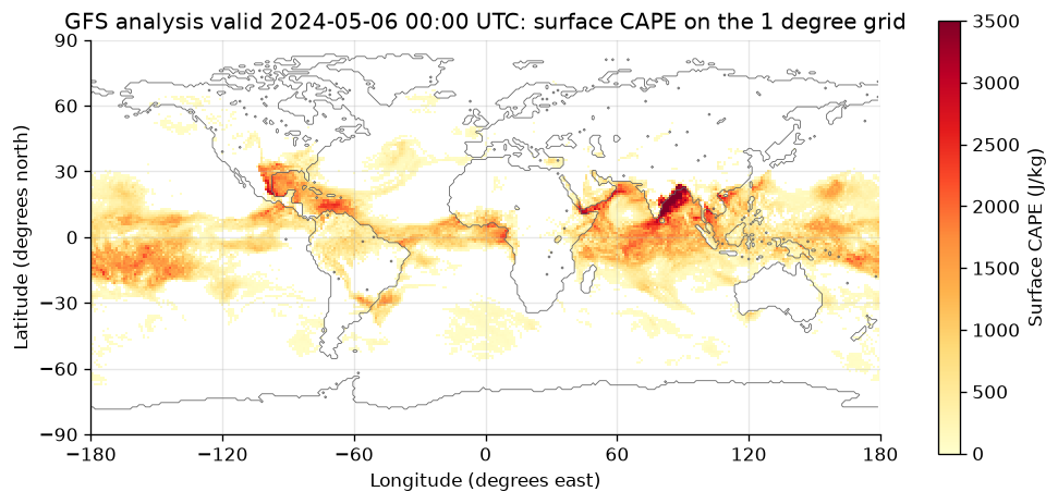

cape = world["cape"]
peak = cape.where(cape == cape.max(), drop=True)
print(f"Largest surface CAPE: {float(cape.max()):.0f} J/kg")
print(f"  at {float(peak.latitude[0]):.0f} N {float(peak.longitude[0]):.0f} E")
unstable = cape >= 1000
tropical = unstable.where(np.abs(world.latitude) < 30, False)
print(f"Grid cells with CAPE >= 1000 J/kg: {int(unstable.sum())}")
print(f"  within 30 degrees of the equator: {int(tropical.sum())}")

Largest surface CAPE: 4096 J/kg
  at 12 N 80 E
Grid cells with CAPE >= 1000 J/kg: 3653
  within 30 degrees of the equator: 3576

At this hour nearly all the instability on Earth sat in the tropics: 3576 of the 3653 cells with at least 1000 J/kg lie within 30 degrees of the equator, and the largest value is over the Bay of Bengal, off the southeast coast of India. The two tongues reaching past 30 degrees are over Texas and the Gulf coast, and over southern Brazil. Cells under 50 J/kg are left blank.

Oklahoma City's cell, a 1 degree box about 100 km across, held 61 J/kg at 7 pm local time on 5 May. The analysis is 28 hours 39 minutes before the Oklahoma County tornado report that the severe-weather case study follows, so it describes the air mass a day earlier, not the environment the storms formed in; the HRRR walkthrough maps the same two fields on a 3 km grid at 20 UTC on 6 May.

Pin and cite

verify checks the cached file against the lockfile's checksum. Keep the manifest, lockfile, and cached bytes together; public cloud retention is not a promise.

assert verify(manifest) == []
for citation in cite_lockfile(manifest):
    print(citation.as_text())

noaa:gfs
  NOAA Global Forecast System (GFS) was accessed on 2026-09-16 from https://registry.opendata.aws/noaa-gfs-bdp-pds
  homepage: https://registry.opendata.aws/noaa-gfs-bdp-pds/
  license: US Government Work (public domain)
  terms: https://www.noaa.gov/information-technology/open-data-dissemination
  retrieved: 2026-09-16; 1 checksummed asset (42,362,644 bytes) pinned by usdata 0.18.0
  sources: 1

What was awkward

Pressure levels come under two level types. Levels from 1000 to 1 hPa are isobaricInhPa, but the eight above them, 0.7 to 0.01 hPa, are isobaricInPa with levels numbered in pascals, so a select for every temperature level with typeOfLevel: isobaricInhPa misses eight of them, and 80 messages in all, without saying so.
Two opens and an xr.merge were the simplest way to get CAPE and helicity with short names; one select spanning both level types would rename every variable to shortName_typeOfLevel_level.
Units arrive as raw ecCodes strings, J kg**-1 and m**2 s**-2. Every plot label and sentence translates them by hand.
Longitudes run 0 to 359, so a western place needs % 360 to be found and a map of the Americas needs the coordinates rolled and re-sorted first.
The two dates in this notebook disagree. A pull that restores from the committed lockfile downloads the object again, so retrieved_at above is the day this notebook ran, while the citation says the file was accessed on the day the lockfile was first written. The citation is the one to quote, but nothing on the fetched item says so.
The grib extra installs with pip alone on Linux, and on Windows through Python 3.13; macOS needs the ecCodes library from conda-forge or Homebrew first. The reader reference has the details.

GFS model output

At a glance

Quick start

Walkthrough