usdata
NOAA's Global Summary of the Month (GSOM) condenses each land station's daily GHCN-Daily record into one row per calendar month: total precipitation, mean temperature, extremes, and counts of days past thresholds. NCEI publishes it through its Access Data Service, and one request returns one CSV with a row per station and month.
This walkthrough pulls five years of monthly precipitation and mean
temperature at Will Rogers World Airport in Oklahoma City, January 2020 to
December 2024. It needs usdata[pandas] and matplotlib, and runs in a few
seconds.
from datetime import UTC, datetime
from pathlib import Path

import matplotlib.pyplot as plt
import pandas as pd

import usdata
from usdata import cite_lockfile, pull, verify

# One figure style for every usdata notebook, so previews look alike.
plt.rcParams.update(
    {
        "figure.figsize": (8, 4.5),
        "figure.dpi": 120,
        "axes.spines.top": False,
        "axes.spines.right": False,
        "axes.grid": True,
        "grid.alpha": 0.3,
        "font.size": 10,
    }
)
manifest = Path("dataset.yaml")
print("Executed (UTC):", datetime.now(UTC).isoformat(timespec="seconds"))
print(f"usdata {usdata.__version__}; pandas {pd.__version__}")
Executed (UTC): 2026-09-24T05:55:14+00:00
usdata 0.26.0; pandas 3.0.6
Select
The manifest names one station, two variables, and a window. GSOM selects
every UTC calendar month the window touches, in full: 6 to 7 May selects all
of May, and 31 May to 1 June selects both months. USW00013967 is the
airport's GHCN station ID; a bbox or place in place of stations finds
stations through NCEI's search service. units: metric asks for millimetres
and degrees Celsius.
print(manifest.read_text())name: okc-monthly-climate
sources:
- dataset: noaa:gsom
start: 2020-01-01
end: 2024-12-31
variables: [PRCP, TAVG]
params:
stations: USW00013967
units: metric
What arrives
The first pull downloads one CSV and writes dataset.lock.json beside the
manifest, pinning the file's checksum. Later pulls reuse the pin and the cache.
result = pull(manifest)
(item,) = result.fetched
print("File:", item.path.name)
print("Bytes:", item.provenance.size)
print("Source:", item.provenance.source_url)
print("Retrieved (UTC):", item.provenance.retrieved_at.isoformat(timespec="seconds"))
print("Checksum:", item.provenance.checksum)
File: global-summary-of-the-month_2020-01-01_2024-12-31_de68833a1ecf.csv
Bytes: 4200
Source: https://www.ncei.noaa.gov/access/services/data/v1?dataset=global-summary-of-the-month&stations=USW00013967&startDate=2020-01-01&endDate=2024-12-31&format=csv&units=metric&includeStationLocation=1&dataTypes=PRCP%2CTAVG
Retrieved (UTC): 2026-09-24T05:55:14+00:00
Checksum: sha256:c9d6f9135d27bc26602fd74b00ad9451a00f6985323ffa25da18da6ced04ef8d
Open
The generic CSV reader returns a DataFrame with one row per month. DATE is a
YYYY-MM label for a whole month, not a timestamp; parsing it as a monthly
period keeps that meaning. PRCP is the month's total in millimetres and
TAVG its mean in degrees Celsius. NCEI's CSV has no units row, so the units
come from the request. Each row repeats the station's latitude, longitude, and
elevation in metres.
frame = item.open()
frame["MONTH"] = pd.PeriodIndex(frame["DATE"], freq="M")
print(f"{len(frame)} rows, {frame['MONTH'].min()} to {frame['MONTH'].max()}")
frame[["STATION", "LATITUDE", "LONGITUDE", "ELEVATION", "DATE", "PRCP", "TAVG"]].head()
60 rows, 2020-01 to 2024-12
| STATION | LATITUDE | LONGITUDE | ELEVATION | DATE | PRCP | TAVG | |
|---|---|---|---|---|---|---|---|
| 0 | USW00013967 | 35.38843 | -97.60035 | 389.9 | 2020-01 | 79.8 | 5.9 |
| 1 | USW00013967 | 35.38843 | -97.60035 | 389.9 | 2020-02 | 16.5 | 5.3 |
| 2 | USW00013967 | 35.38843 | -97.60035 | 389.9 | 2020-03 | 127.8 | 13.0 |
| 3 | USW00013967 | 35.38843 | -97.60035 | 389.9 | 2020-04 | 51.5 | 14.1 |
| 4 | USW00013967 | 35.38843 | -97.60035 | 389.9 | 2020-05 | 103.7 | 19.8 |
A first look
The same twelve calendar months, five times over: each year's monthly mean temperature as a line, and each year's monthly precipitation as a dot beside the five-year median.
frame["YEAR"] = frame["MONTH"].dt.year
frame["CALENDAR_MONTH"] = frame["MONTH"].dt.month
labels = ["J", "F", "M", "A", "M", "J", "J", "A", "S", "O", "N", "D"]
years = sorted(frame["YEAR"].unique())
shades = plt.cm.viridis([i / (len(years) - 1) for i in range(len(years))])

fig, (warm, wet) = plt.subplots(2, 1, sharex=True, layout="constrained")
for year, shade in zip(years, shades, strict=True):
    rows = frame[frame["YEAR"] == year]
    warm.plot(rows["CALENDAR_MONTH"], rows["TAVG"], color=shade, linewidth=1.2, label=str(year))
    wet.scatter(rows["CALENDAR_MONTH"], rows["PRCP"], color=shade, s=18, zorder=3)
median = frame.groupby("CALENDAR_MONTH")["PRCP"].median()
wet.bar(
    median.index, median.values, color="#2563a6", alpha=0.25, width=0.7, label="Five-year median"
)
warm.set_ylabel("Mean temperature (°C)")
warm.set_title("Will Rogers World Airport, Oklahoma City: monthly summaries, 2020 to 2024")
warm.legend(ncols=5, fontsize=8, loc="upper left", frameon=False)
wet.set_ylabel("Precipitation (mm)")
wet.legend(fontsize=8, loc="upper left", frameon=False)
wet.set_xticks(range(1, 13), labels)
wet.set_xlabel("Calendar month")
plt.show()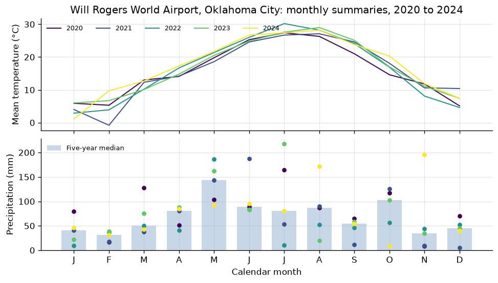
spread = frame.groupby("CALENDAR_MONTH").agg(
    TAVG_RANGE=("TAVG", lambda values: values.max() - values.min()),
    PRCP_MIN=("PRCP", "min"),
    PRCP_MAX=("PRCP", "max"),
)
calm, rough = spread["TAVG_RANGE"].idxmin(), spread["TAVG_RANGE"].idxmax()
widest = spread["PRCP_MAX"].sub(spread["PRCP_MIN"]).idxmax()
print(
    "Year-to-year range of the monthly mean temperature: "
    f"{spread.loc[calm, 'TAVG_RANGE']:.1f} °C in month {calm}, "
    f"{spread.loc[rough, 'TAVG_RANGE']:.1f} °C in month {rough}"
)
print(
    f"Precipitation in month {widest} ranged {spread.loc[widest, 'PRCP_MIN']:.1f} to "
    f"{spread.loc[widest, 'PRCP_MAX']:.1f} mm across the five years"
)
Year-to-year range of the monthly mean temperature: 2.1 °C in month 6, 10.5 °C in month 2
Precipitation in month 7 ranged 10.7 to 217.9 mm across the five years
The seasonal cycle, more than 20 °C from January to July, repeats closely in summer: June's mean stayed within about 2 °C across the five years. Winter varies more, with February 2021 below freezing and February 2024 near 10 °C. Precipitation is far less regular: one calendar month can differ twentyfold between years. Five years at one station show that spread; they are not a climate normal, which the Climate Normals dataset provides for 1991 to 2020.
Pin and cite
verify checks the cached file against the lockfile's checksum. Keep the
manifest and lockfile with your analysis; the citation below is what a
methods section needs, and usdata cite dataset.yaml prints the same.
assert verify(manifest) == []
for citation in cite_lockfile(manifest):
    print(citation.as_text())
noaa:gsom
Lawrimore, Jay H.; Ray, Ron; Applequist, Scott; Korzeniewski, Bryant; Menne, Matthew J. (2016): Global Summary of the Month (GSOM), Version 1. NOAA National Centers for Environmental Information. https://doi.org/10.7289/V5QV3JJ5
homepage: https://www.ncei.noaa.gov/access/search/data-search/global-summary-of-the-month
license: US Government Work (public domain)
terms: https://www.ncei.noaa.gov/metadata/geoportal/rest/metadata/item/gov.noaa.ncdc:C00946/html
retrieved: 2026-09-24; 1 checksummed asset (4,200 bytes) pinned by usdata 0.26.0
sources: 1
What was awkward
- The CSV carries no units. The request's
units: metricis the only record of whetherPRCPis millimetres or inches, so the manifest has to travel with the data. - The window widens to whole UTC months without saying so. A query for one week in May returns the May row, and the asset's time bounds cover all of May rather than the dates asked for.
DATEis text such as2024-05. Grouping by calendar month needs a parse first;pd.PeriodIndex(..., freq="M")keeps it a month rather than pretending it is the first day of one.- Changing the window in a locked manifest is reported as an input change
until the pull is repeated with
force=True, which replaces the lockfile. That protects the pin but is a step to remember when exploring.